[Avg. reading time: 0 minutes]

[Avg. reading time: 2 minutes]
Disclaimer

1. Week 1 > 2. Week 8 > 3. Week 15
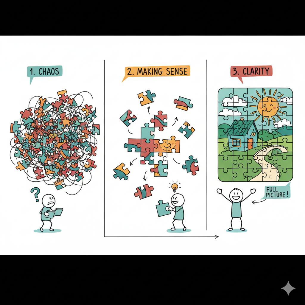
In this AI era, remember the following.
- First, you are not behind, you are learning on schedule.
- Second, feeling like an imposter is normal, it means you are stretching your skills.
- Third, ignore the online noise. Learning is simple: learn something, think about it, practice it, repeat.
- Lastly, tools will change, but your ability to learn will stay.
Certificates are good, but projects and understanding matter more. Ask questions, help each other, and don’t do this journey alone.
[Avg. reading time: 2 minutes]
Required Tools
Install these softwares before Week 2.
Windows
Mac
Common Tools (Windows & Mac)
-
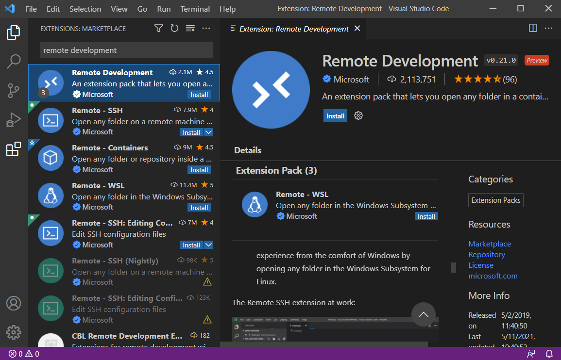
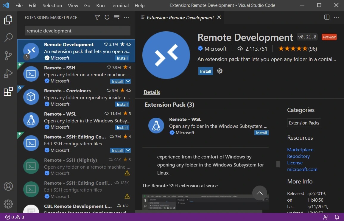
Install this VS Code Extension
Remote Development
[Avg. reading time: 13 minutes]
Setting up Bigdata Environment
This setup creates a ready-made development environment for this course.
Instead of installing the necessary softwares, libraries, compilers, and tools on your laptop, everything runs inside a container.
This guarantees everyone has the exact same setup, so there’s no “it works on my machine” problem.
We will learn how this works in later weeks.
Video
Step by Step
- Install VSCode and Remote Development Extension
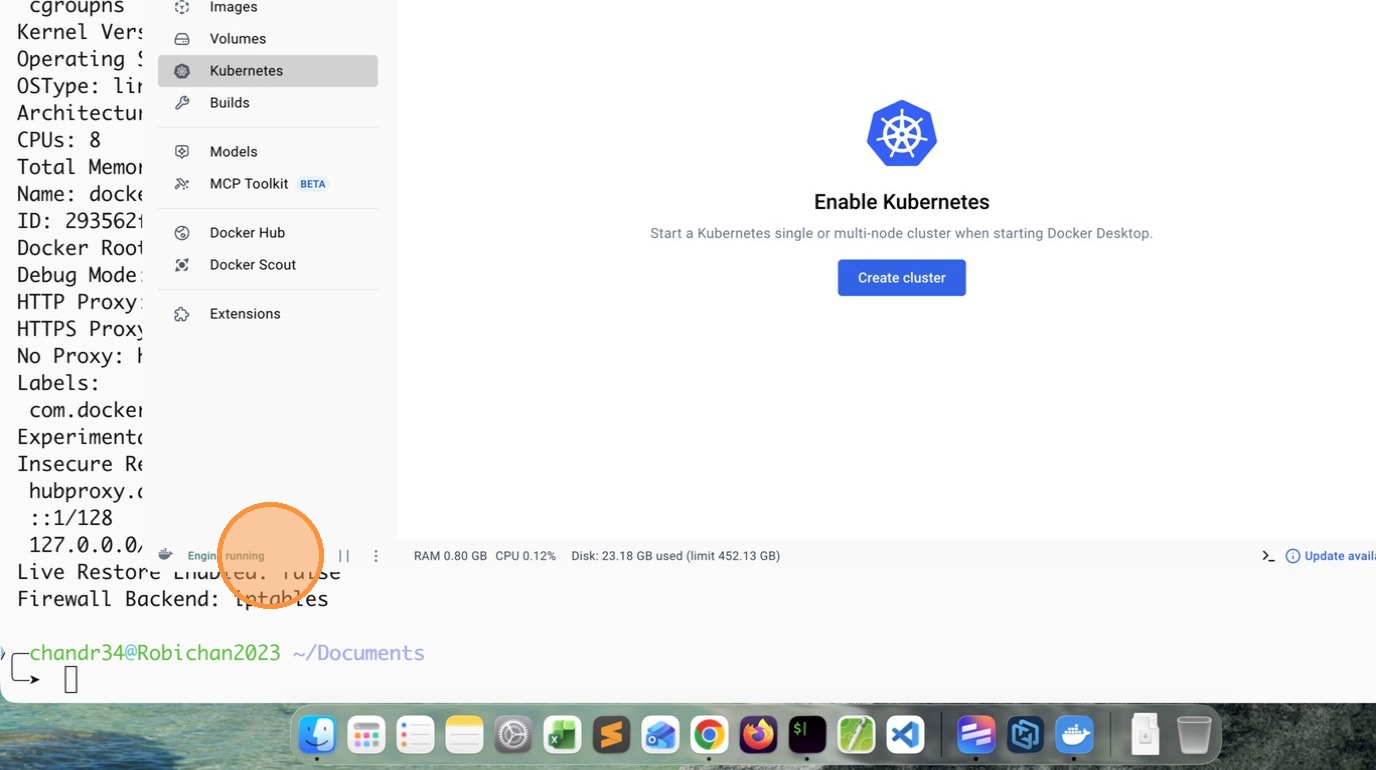
- Install Docker Personal and make sure Engine is running
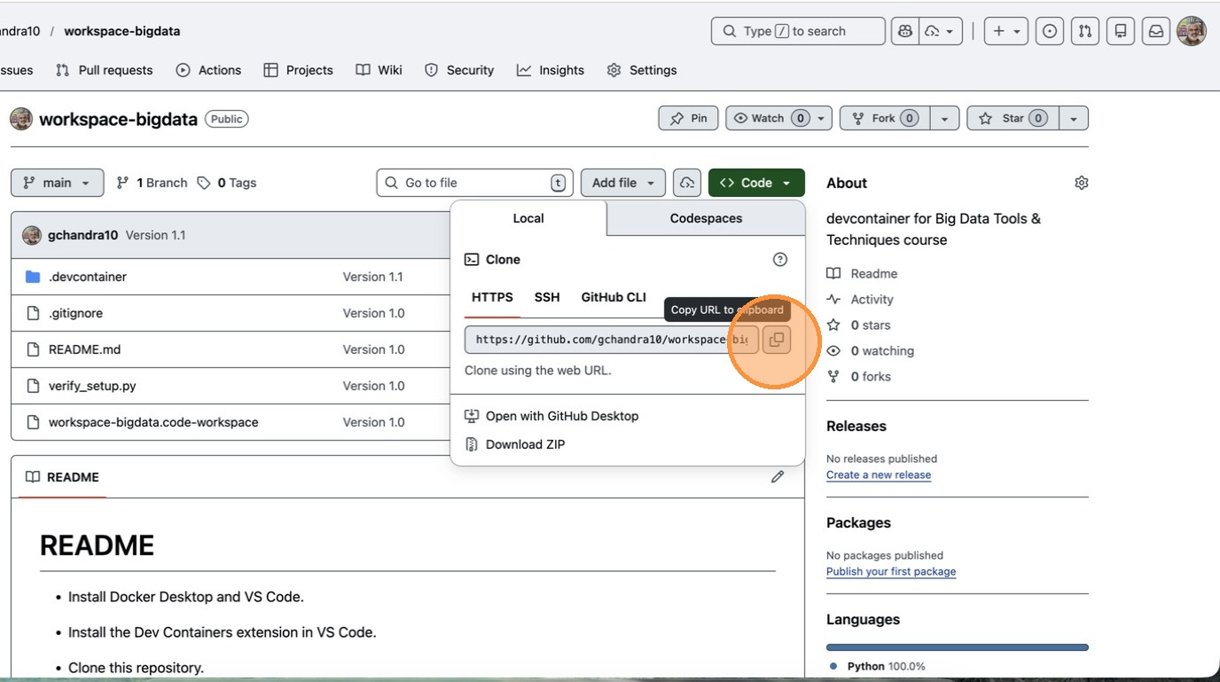
- Copy the gitrepo https://github.com/gchandra10/workspace-bigdata
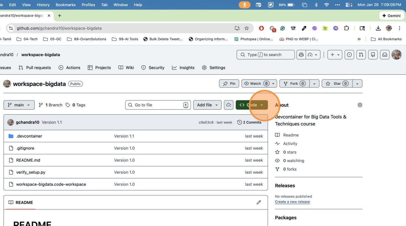
- Click “Copy URL to clipboard”
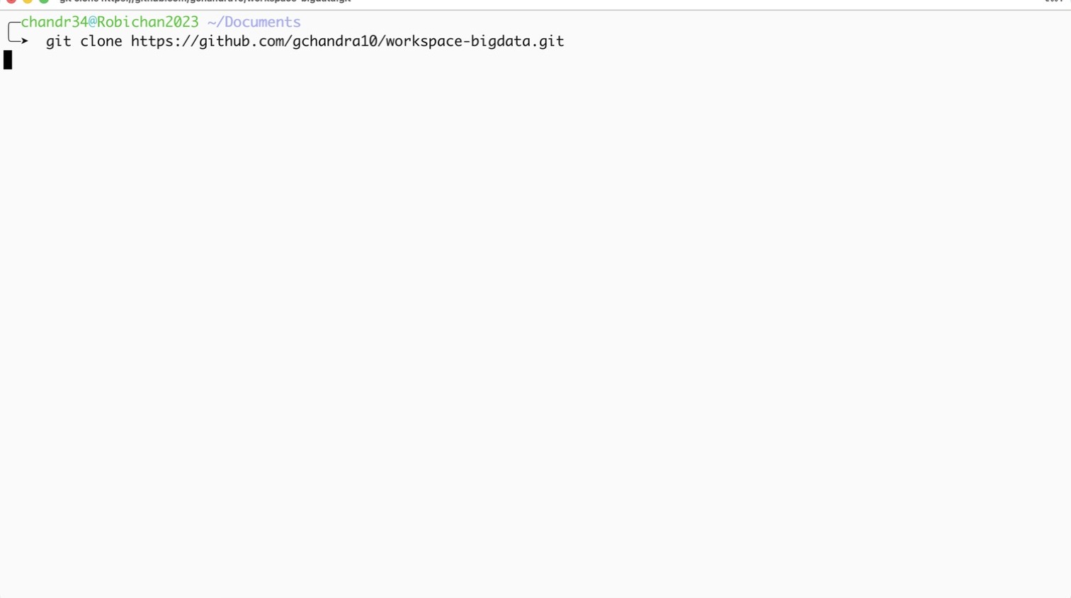
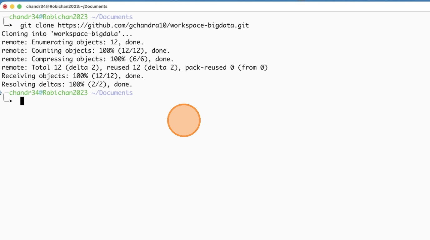
- Open Terminal / Command Prompt and clone the Repo
- Step after cloning the repo
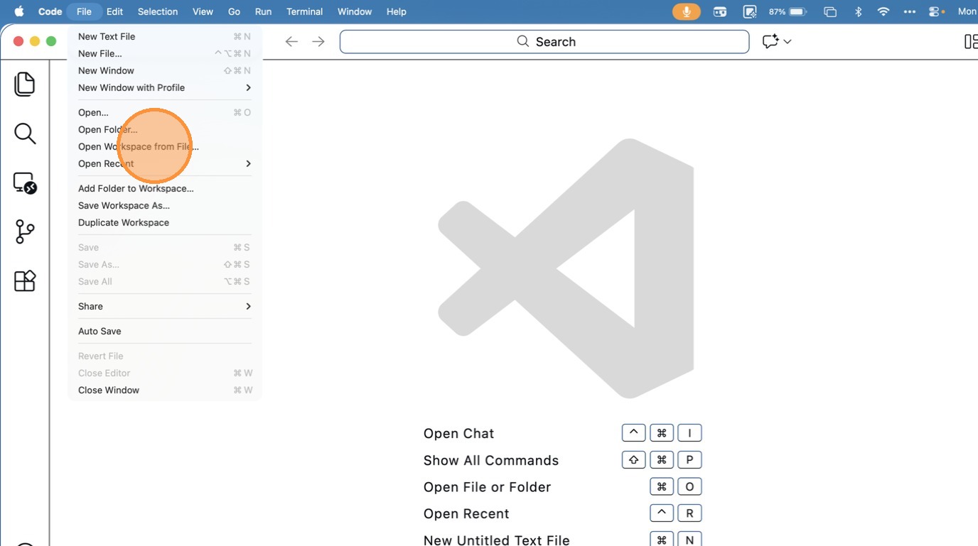
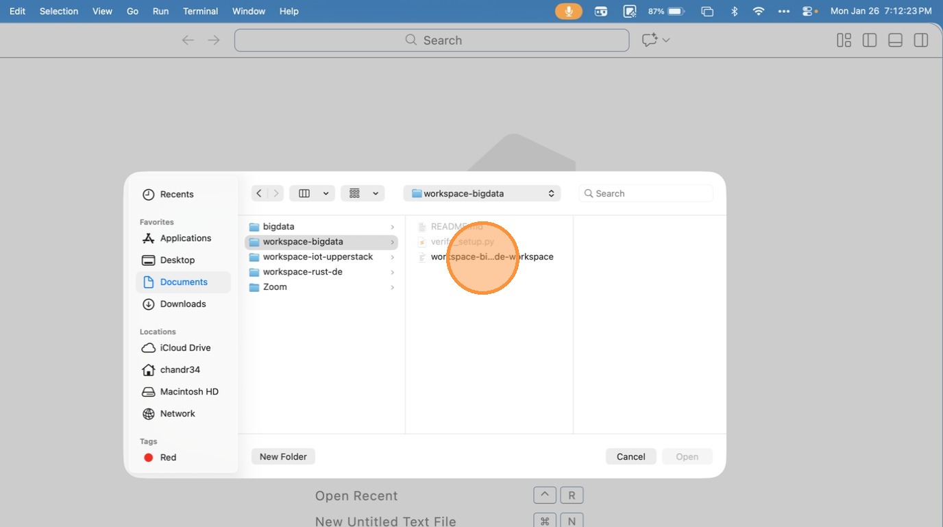
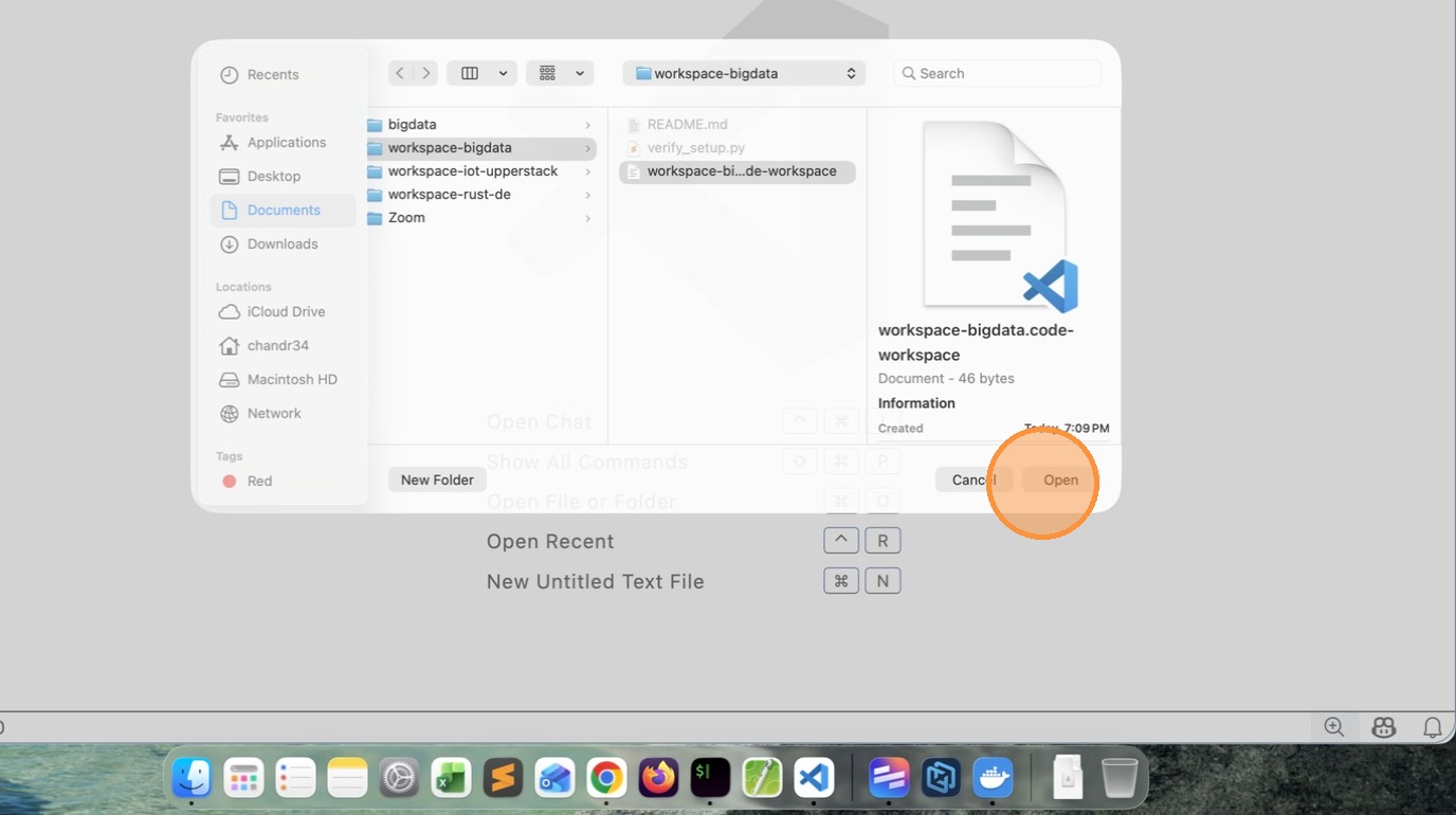
- Click “Open Workspace from File…”
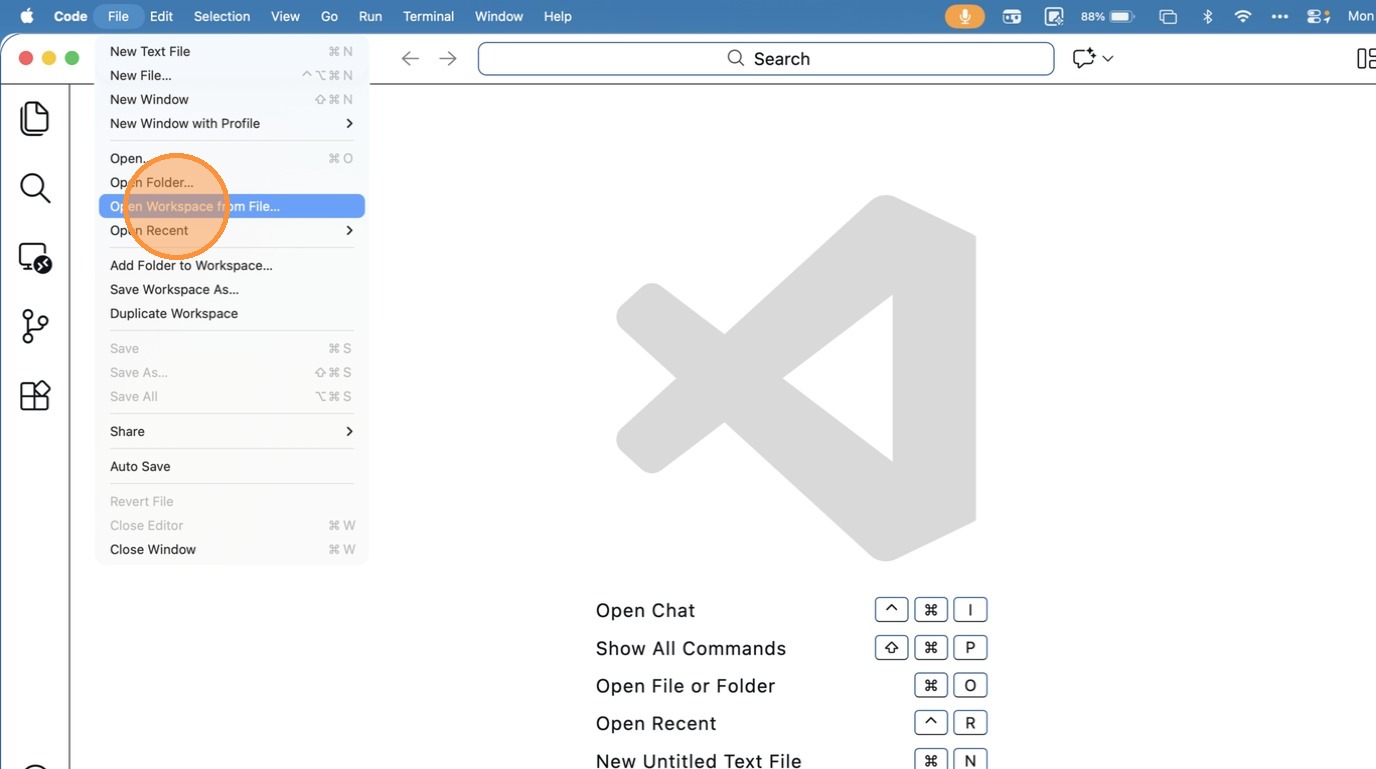
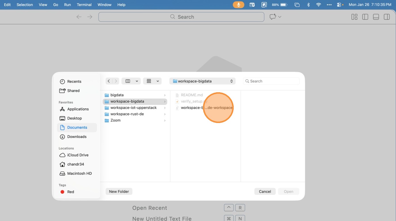
- Choose the Workspace file inside the folder
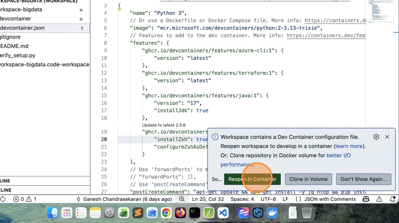
- VSCode will prompt to Reopen in Container, click that Button.
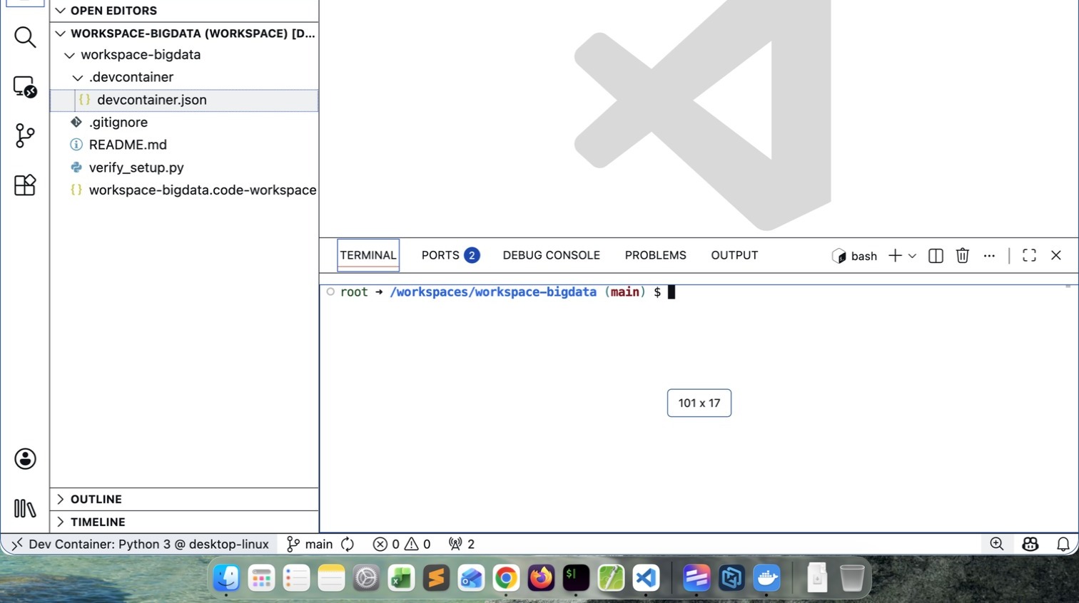
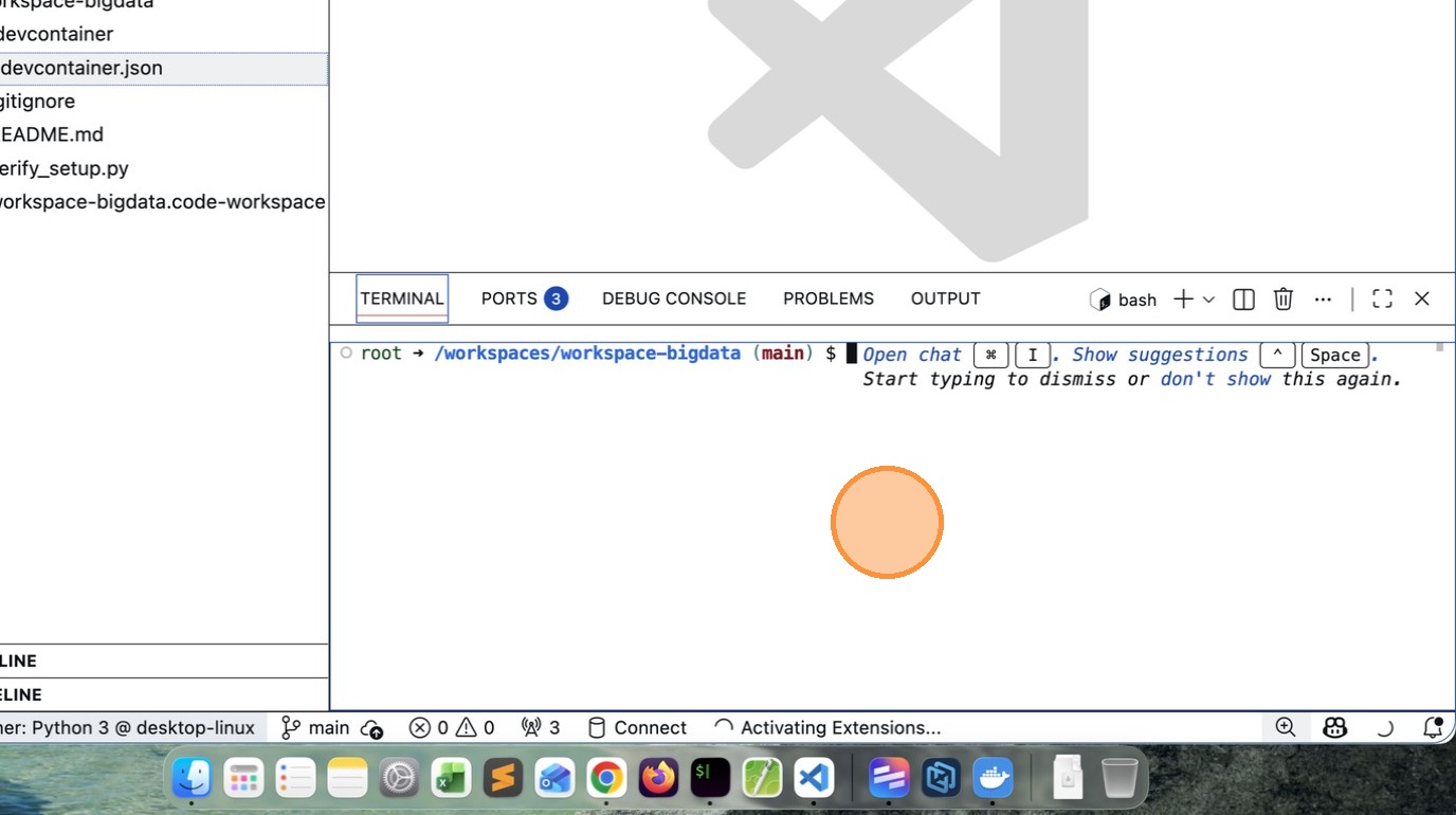
- After few minutes (depends on your computer capability and network speed), you will see a message like this.
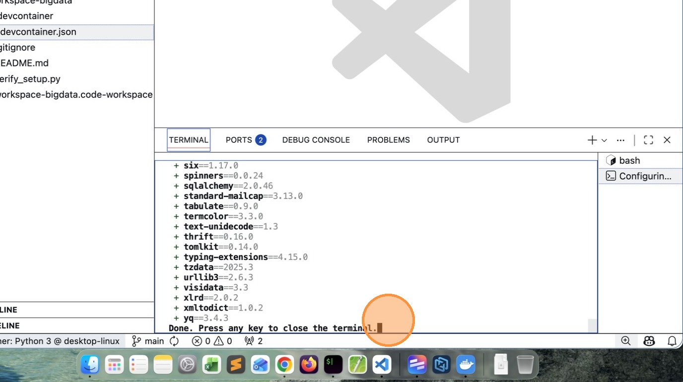
- If you see /workspaces/workspace-bigdata $ your installation is successful
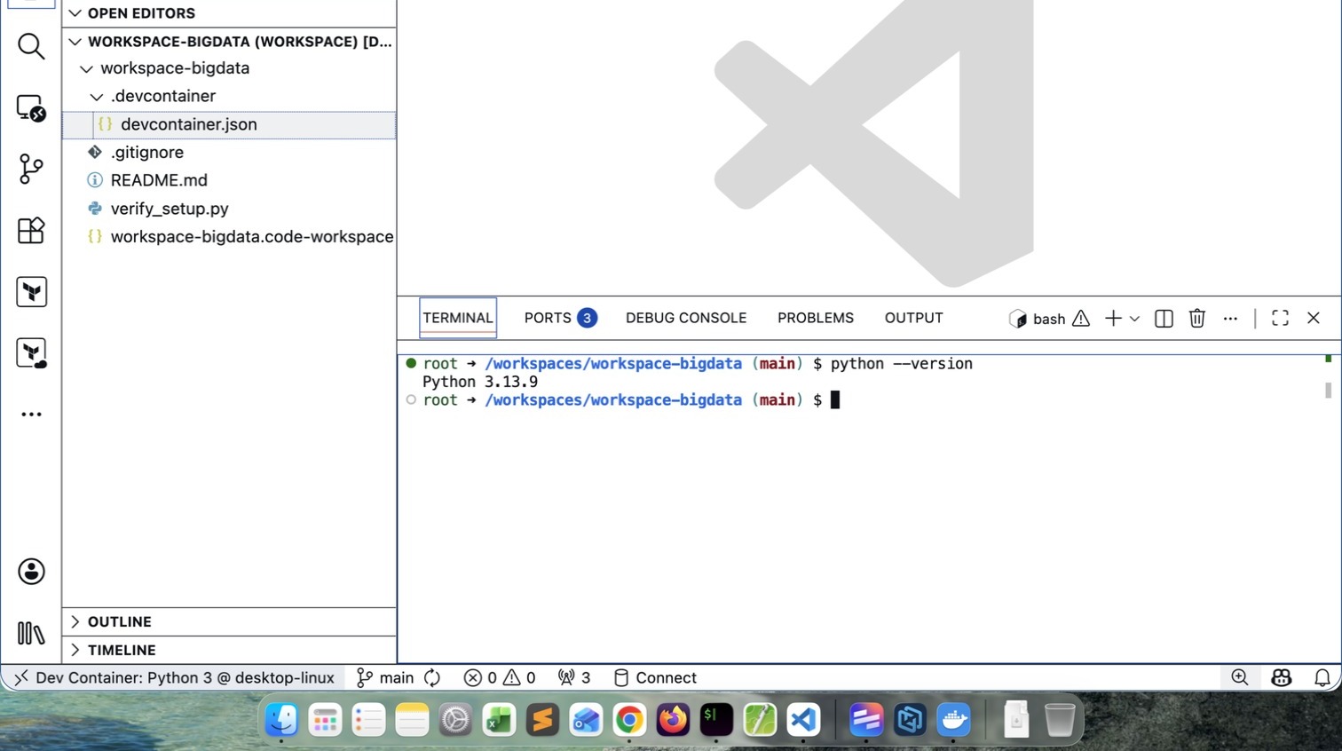
- Verify the Python version. It may vary depending upon what is latest at that time.
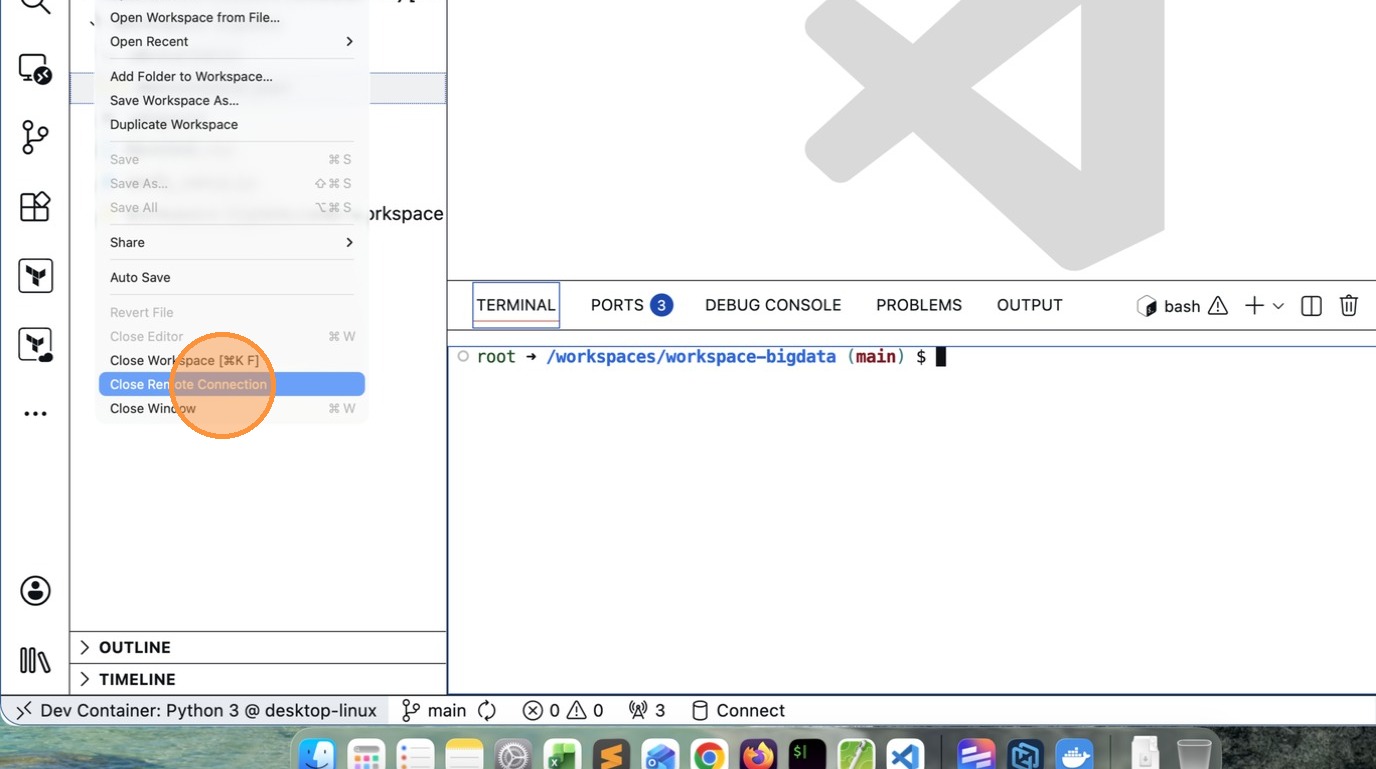
How to close the Workspace
- Click “Close Remote Connection”
How to ReOpen Workspace again
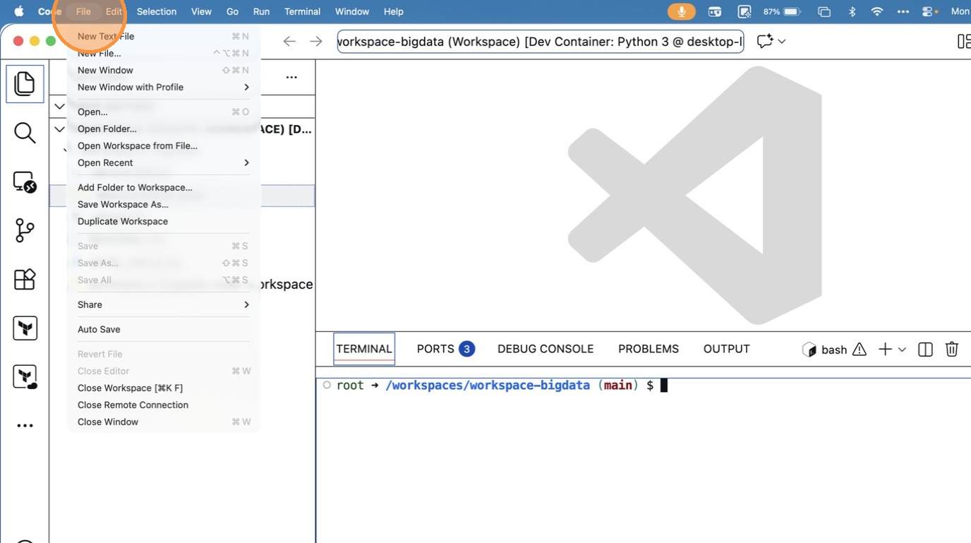
- Click “File”
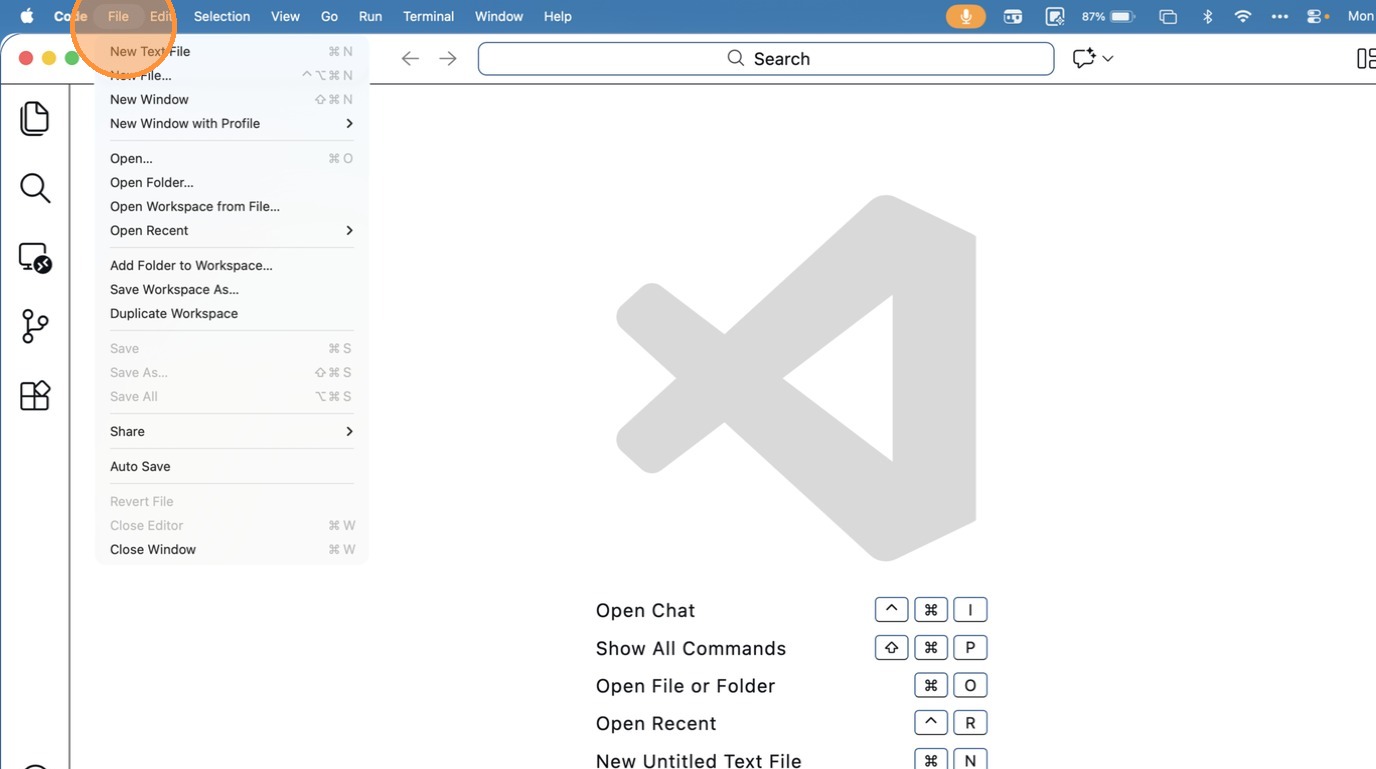
- Click “Open Workspace from File…”
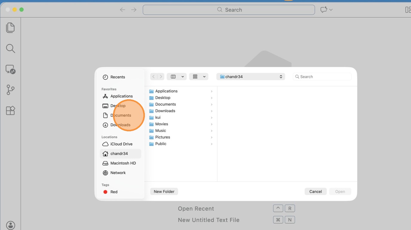
- Click “Documents”
- Click “text field”
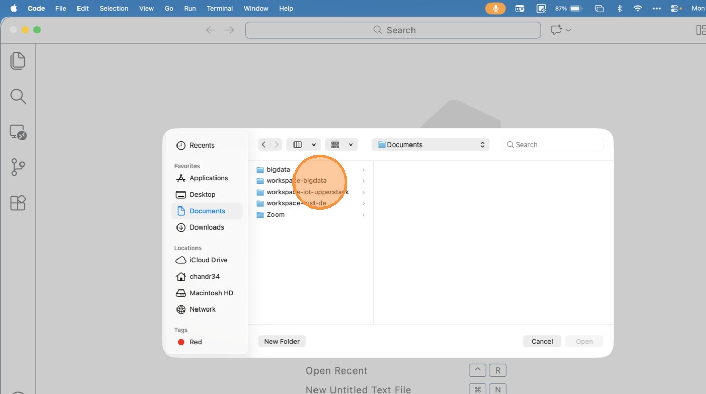
- Click “text field”
- Click “open workspace from file”
Tip: This time it will load the Remote Workspace immediately.
- Click “image”
Reset and Retry
- Close VSCode
- Delete workspace-bigdata folder and all files
- Open command prompt
- Run the following commands to clean the existing containers
docker rm $(docker ps -aq)

docker rmi $(docker image -aq)

docker volume rm $(docker volume ls -q)
- Goto command prompt clone the repository (I have updated a newer version)
https://github.com/gchandra10/workspace-bigdata.git
And follow the steps mentioned above
Note: pls make sure docker is running and you have enough space.
#setup #workspace #devcontainer
[Avg. reading time: 3 minutes]
Big Data Overview
- Introduction
- Job Opportunities
- What is Data?
- How does it help?
- Types of Data
- The Big V’s
- Trending Technologies
- Big Data Concerns
- Big Data Challenges
- Data Integration
- Scaling
- CAP Theorem
- PACELC Theorem
- Optimistic Concurrency
- Eventual Consistency
- Concurrent vs Parallel
- GPL
- DSL
- Big Data Tools
- NO Sql Databases
- Learning Big Data means?
#introduction #bigdata #chapter1
[Avg. reading time: 2 minutes]
Understanding the Big Data Landscape
Expectation in this course
The first set of questions, which everyone is curious to know.
What is Big Data?
When does the data become Big Data?
Why collect so much Data?
How secure is Big Data?
How does it help?
Where can it be stored?
Which Tools are used to handle Big Data?
The second set of questions to get in deep.
What should I learn?
Does certification help?
Which technology is the best?
How many tools do I need to learn?
Apart from the top 50 corporations, do other companies use Big Data?
[Avg. reading time: 3 minutes]
Job Opportunities
| Role | On-Prem | Big Data Specific | Cloud |
|---|---|---|---|
| Database Developer | ✅ | ✅ | ✅ |
| Data Engineer | ✅ | ✅ | ✅ |
| Database Administrator | ✅ | ✅ | ✅ |
| Data Architect | ✅ | ✅ | ✅ |
| Database Security Eng. | ✅ | ✅ | ✅ |
| Database Manager | ✅ | ✅ | ✅ |
| Data Analyst | ✅ | ✅ | ✅ |
| Business Intelligence | ✅ | ✅ | ✅ |
Database Developer: Designs and writes efficient queries, procedures, and data models for structured databases.
Data Engineer: Builds and maintains scalable data pipelines and ETL processes for large-scale data movement and transformation.
Database Administrator (DBA): Manages and optimizes database systems, ensuring performance, security, and backups.
Data Architect: Defines high-level data strategy and architecture, ensuring alignment with business and technical needs.
Database Security Engineer: Implements and monitors security controls to protect data assets from unauthorized access and breaches.
Database Manager: Oversees database teams and operations, aligning database strategy with organizational goals.
Data Analyst: Interprets data using statistical tools to generate actionable insights for decision-makers.
Business Intelligence (BI) Developer: Creates dashboards, reports, and visualizations to help stakeholders understand data trends and KPIs.
All small to enterprise organizations use Big data to develop their business.
[Avg. reading time: 4 minutes]
What is Data?
Data is simply facts and figures. When processed and contextualized, data becomes information.
Everything is data
- What we say
- Where we go
- What we do
How to measure data?
byte        - 1 letter
1 Kilobyte  - 1024 B
1 Megabyte  - 1024 KB
1 Gigabyte  - 1024 MB
1 Terabyte  - 1024 GB
(1,099,511,627,776 Bytes)
1 Petabyte  - 1024 TB
1 Exabyte   - 1024 PB
1 Zettabyte - 1024 EB
1 Yottabyte - 1024 ZB
Examples of Traditional Data
- Banking Records
- Student Information
- Employee Profiles
- Customer Details
- Sales Transactions
When Data becomes Big Data?
When data expands
- Banking: One bank branch vs. global consolidation (e.g., CitiBank)
- Education: One college vs. nationwide student data (e.g., US News)
- Media: Traditional news vs. user-generated content on Social Media
When data gets granular
- Monitoring CPU/Memory usage every second
- Cell phone location & usage logs
- IoT sensor telemetry (temperature, humidity, etc.)
- Social media posts, reactions, likes
- Live traffic data from vehicles and sensors
These fine-grained data points fuel powerful analytics and real-time insights.
Why Collect So Much Data?
- Storage is cheap and abundant
- Tech has advanced to process massive data efficiently
- Businesses use data to innovate, predict trends, and grow
#data #bigdata #traditionaldata
[Avg. reading time: 3 minutes]
How Big Data helps us
From raw blocks to building knowledge, Big Data drives global progress.
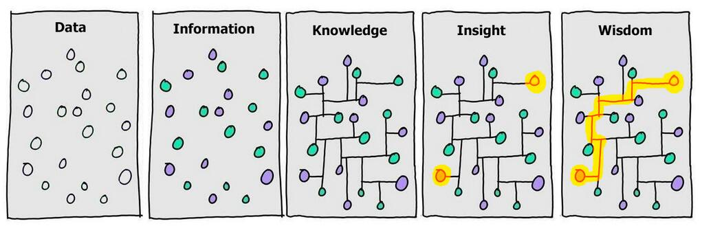
Stages
- Data → scattered observations
- Information → contextualized
- Knowledge → structured relationships
- Insight → patterns emerge
- Wisdom → actionable strategy
Raw Data to Analysis
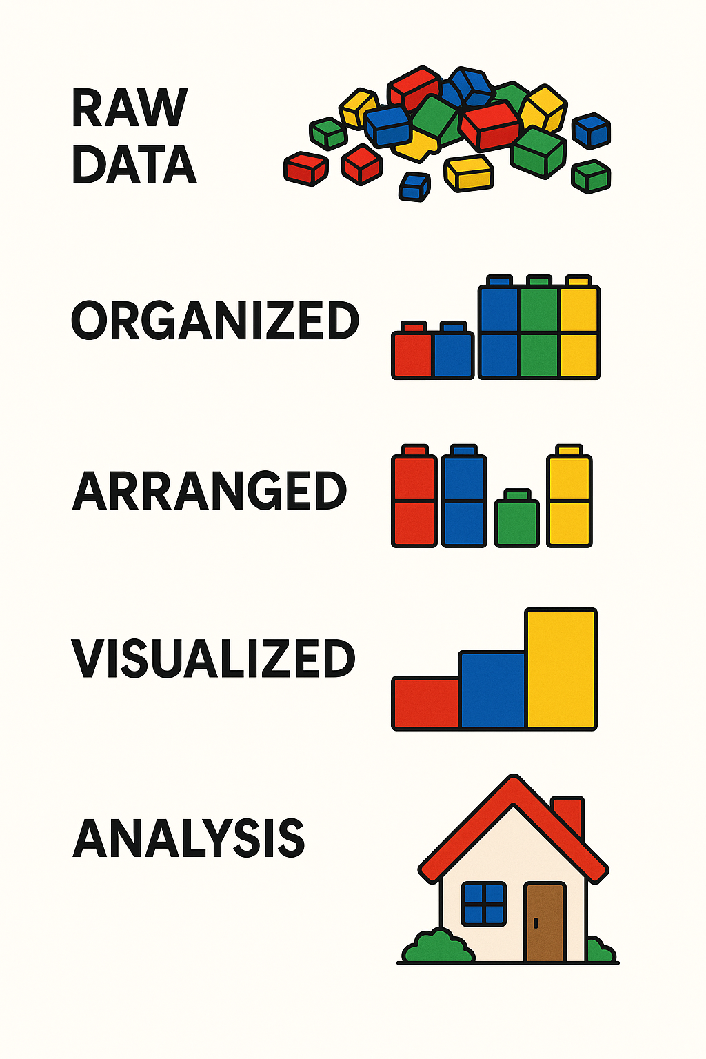
Stages
- Raw Data – Messy, unprocessed
- Organized – Grouped by category
- Arranged – Structured to show comparisons
- Visualized – Charts or graphs
- Analysis – Final understanding or solution
Big Data Applications: Changing the World
Here are some real-world domains where Big Data is making a difference:
- Healthcare – Diagnose diseases earlier and personalize treatment
- Agriculture – Predict crop yield and detect pest outbreaks
- Space Exploration – Analyze signals from space and optimize missions
- Disaster Management – Forecast earthquakes, floods, and storms
- Crime Prevention – Predict and detect crime patterns
- IoT & Smart Devices – Real-time decision making in smart homes, vehicles, and cities
#bigdata #rawdata #knowledge #analysis
[Avg. reading time: 7 minutes]
Types of Data
Understanding the types of data is key to processing and analyzing it effectively. Broadly, data falls into two main categories: Quantitative and Qualitative.
Quantitative Data
Quantitative data deals with numbers and measurable forms. It can be further classified as Discrete or Continuous.
- Measurable values (e.g., memory usage, CPU usage, number of likes, shares, retweets)
- Collected from the real world
- Usually close-ended
Discrete
- Represented by whole numbers
- Countable and finite
Example:
- Number of cameras in a phone
- Memory size in GB
Qualitative Data
Qualitative data describes qualities or characteristics that can’t be easily measured numerically.
- Descriptive or abstract
- Can come from text, audio, or images
- Collected via interviews, surveys, or observations
- Usually open-ended
Examples
- Gender: Male, Female, Non-Binary, etc.
- Smartphones: iPhone, Pixel, Motorola, etc.
Nominal
Categorical data without any intrinsic order
Examples:
- Red, Blue, Green
- Types of fruits: Apple, Banana, Mango
Can you rank them logically? No — that’s what makes them nominal.
graph TD
  A[Types of Data]

  A --> B[Quantitative]
  A --> C[Qualitative]

  B --> B1[Discrete]
  B --> B2[Continuous]

  C --> C1[Nominal]
  C --> C2[Ordinal]
| Category | Subtype | Description | Examples |
|---|---|---|---|
| Quantitative | Discrete | Whole numbers, countable | Number of phones, number of users |
| Continuous | Measurable, can take fractional values | Temperature, CPU usage | |
| Qualitative | Nominal | Categorical with no natural order | Gender, Colors (Red, Blue, Green) |
| Ordinal | Categorical with a meaningful order | T-shirt sizes (S, M, L), Grades (A, B, C…) |
Abstract Understanding
Some qualitative data comes from non-traditional sources like:
- Conversations
- Audio or video files
- Observations or open-text survey responses
This type of data often requires interpretation before it’s usable in models or analysis.

#quantitative #qualitative #discrete #continuous #nominal #ordinal
[Avg. reading time: 1 minute]
The Big V’s of Big Data
[Avg. reading time: 7 minutes]
Variety
Variety refers to the different types, formats, and sources of data collected — one of the 5 Vs of Big Data.
Types of Data : By Source
- Social Media: YouTube, Facebook, LinkedIn, Twitter, Instagram
- IoT Devices: Sensors, Cameras, Smart Meters, Wearables
- Finance/Markets: Stock Market, Cryptocurrency, Financial APIs
- Smart Systems: Smart Cars, Smart TVs, Home Automation
- Enterprise Systems: ERP, CRM, SCM Logs
- Public Data: Government Open Data, Weather Stations
Types of Data : By Data format
- Structured Data – Organized in rows and columns (e.g., CSV, Excel, RDBMS)
- Semi-Structured Data – Self-describing but irregular (e.g., JSON, XML, Avro, YAML)
- Unstructured Data – No fixed schema (e.g., images, audio, video, emails)
- Binary Data – Encoded, compressed, or serialized data (e.g., Parquet, Protocol Buffers, images, MP3)
Generally unstructured data files are stored in binary format, Example: Images, Video, Audio
But not all binary files contain unstructured data. Example: Parquet, Executable.
Structured Data
Tabular data from databases, spreadsheets.
Example:
- Relational Table
- Excel
| ID | Name | Join Date |
|---|---|---|
| 101 | Rachel Green | 2020-05-01 |
| 201 | Joey Tribianni | 1998-07-05 |
| 301 | Monica Geller | 1999-12-14 |
| 401 | Cosmo Kramer | 2001-06-05 |
Semi-Structred Data
Data with tags or markers but not strictly tabular.
JSON
[
   {
      "id":1,
      "name":"Rachel Green",
      "gender":"F",
      "series":"Friends"
   },
   {
      "id":"2",
      "name":"Sheldon Cooper",
      "gender":"M",
      "series":"BBT"
   }
]
XML
<?xml version="1.0" encoding="UTF-8"?>
<actors>
   <actor>
      <id>1</id>
      <name>Rachel Green</name>
      <gender>F</gender>
      <series>Friends</series>
   </actor>

   <actor>
      <id>2</id>
      <name>Sheldon Cooper</name>
      <gender>M</gender>
      <series>BBT</series>
   </actor>
</actors>
Unstructured Data
Media files, free text, documents, logs – no predefined structure.
Rachel Green acted in Friends series. Her role is very popular.
Similarly Sheldon Cooper acted in BBT. He acted as nerd physicist.
Types:
- Images (JPG, PNG)
- Video (MP4, AVI)
- Audio (MP3, WAV)
- Documents (PDF, DOCX)
- Emails
- Logs (system logs, server logs)
- Web scraping content (HTML, raw text)
Note: Now we have lot of LLM (AI tools) that helps us parse Unstructured Data into tabular data quickly.
#structured #unstructured #semistructured #binary #json #xml #image #bigdata #bigv
[Avg. reading time: 4 minutes]
Volume
Volume refers to the sheer amount of data generated every second from various sources around the world. It’s one of the core characteristics that makes data big.With the rise of the internet, smartphones, IoT devices, social media, and digital services, the amount of data being produced has reached zettabyte and soon yottabyte scales.
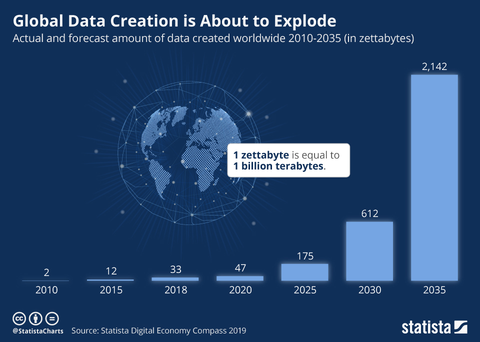
- YouTube users upload 500+ hours of video every minute.
- Facebook generates 4 petabytes of data per day.
- A single connected car can produce 25 GB of data per hour.
- Enterprises generate terabytes to petabytes of log, transaction, and sensor data daily.
Why It Matters
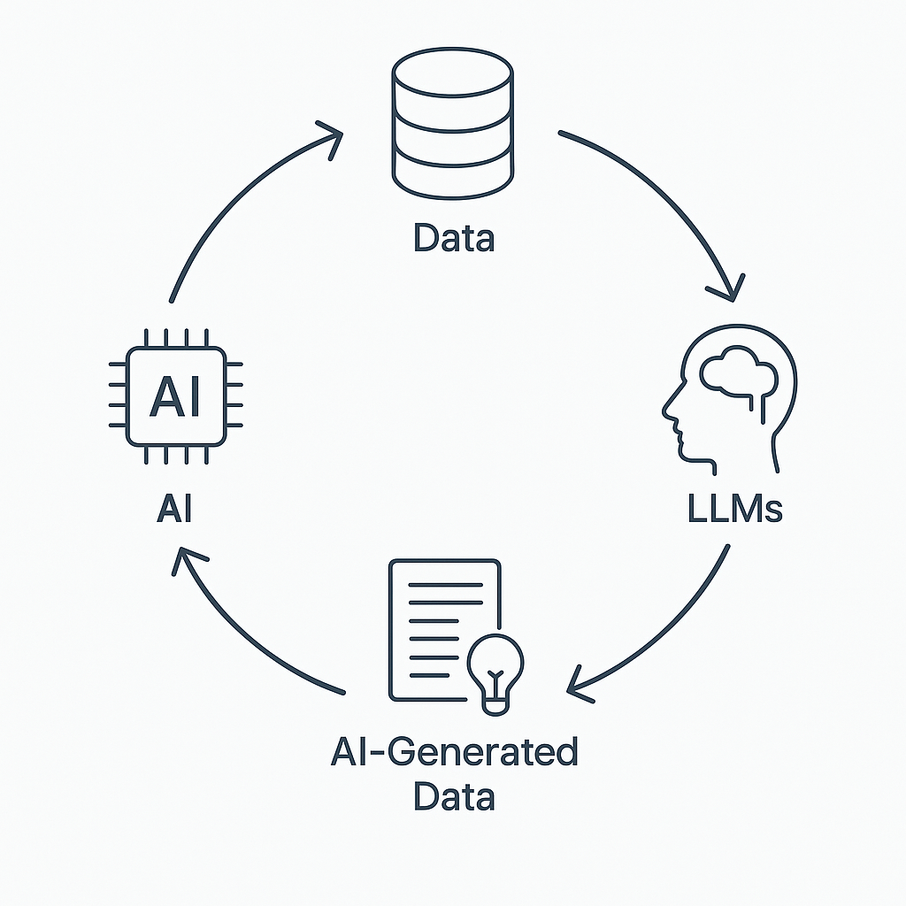
With the rise of Artificial Intelligence (AI) and especially Large Language Models (LLMs) like ChatGPT, Bard, and Claude, the volume of data being generated, consumed, and required for training is skyrocketing.
-
LLMs Need Massive Training Data
-
LLMs generated content is exponential — blogs, reports, summaries, images, audio, and even code.
-
Storage systems must scale horizontally to handle petabytes or more.
-
Traditional databases can’t manage this scale efficiently.
-
Volume impacts data ingestion, processing speed, query performance, and cost.
-
It influences how data is partitioned, replicated, and compressed in distributed systems.
[Avg. reading time: 4 minutes]
Velocity
Velocity refers to the speed at which data is generated, transmitted, and processed. In the era of Big Data, it’s not just about handling large volumes of data, but also about managing the continuous and rapid flow of data in real-time or near real-time.
High-velocity data comes from various sources such as:
- Social Media Platforms: Tweets, posts, likes, and shares occurring every second.
- Sensor Networks: IoT devices transmitting data continuously.
- Financial Markets: Real-time transaction data and stock price updates.
- Online Streaming Services: Continuous streaming of audio and video content.
- E-commerce Platforms: Real-time tracking of user interactions and transactions.
Managing this velocity requires systems capable of:
- Real-Time Data Processing: Immediate analysis and response to incoming data.
- Scalability: Handling increasing data speeds without performance degradation.
- Low Latency: Minimizing delays in data processing and response times.
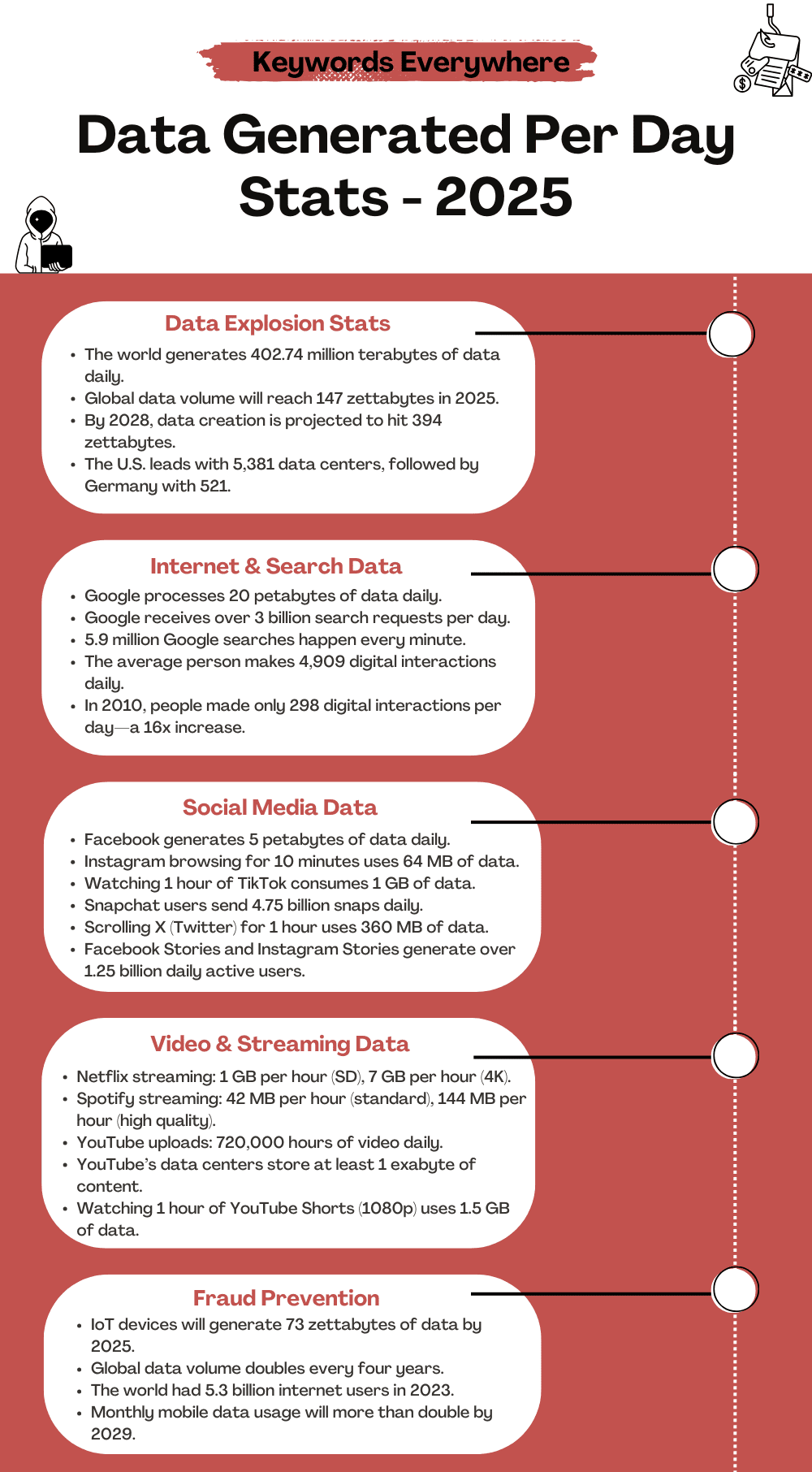 Source1
1: https://keywordseverywhere.com/blog/data-generated-per-day-stats/
[Avg. reading time: 7 minutes]
Veracity
Veracity refers to the trustworthiness, quality, and accuracy of data. In the world of Big Data, not all data is created equal — some may be incomplete, inconsistent, outdated, or even deliberately false. The challenge is not just collecting data, but ensuring it’s reliable enough to make sound decisions.
Why Veracity Matters
-
Poor data quality can lead to wrong insights, flawed models, and bad business decisions.
-
With increasing sources (social media, sensors, web scraping), there’s more noise than ever.
-
Real-world data often comes with missing values, duplicates, biases, or outliers.
Key Dimensions of Veracity in Big Data
| Dimension | Description | Example |
|---|---|---|
| Trustworthiness | Confidence in the accuracy and authenticity of data. | Verifying customer feedback vs. bot reviews |
| Origin | The source of the data and its lineage or traceability. | Knowing if weather data comes from reliable source |
| Completeness | Whether the dataset has all required fields and values. | Missing values in patient health records |
| Integrity | Ensuring the data hasn’t been altered, corrupted, or tampered with during storage or transfer. | Using checksums to validate data blocks |
How to Tackle Veracity Issues
- Data Cleaning: Remove duplicates, correct errors, fill missing values.
- Validation & Verification: Check consistency across sources.
- Data Provenance: Track where the data came from and how it was transformed.
- Bias Detection: Identify and reduce systemic bias in training datasets.
- Robust Models: Build models that can tolerate and adapt to noisy inputs.
Websites & Tools to Generate Sample Data
Highly customizable fake data generator; supports exporting as CSV, JSON, SQL. https://mockaroo.com
Easy UI to create datasets with custom fields like names, dates, numbers, etc. https://www.onlinedatagenerator.com
Apart from this, there are few Data generating libraries.
https://faker.readthedocs.io/en/master/
https://github.com/databrickslabs/dbldatagen
Question?
Is generating fake data good or bad?
When we have real data? why generate fake data?
[Avg. reading time: 3 minutes]
Other V’s in Big Data
| Other V’s | Meaning | Key Question / Use Case |
|---|---|---|
| Value | Business/Customer Impact | What value does this data bring to the business or end users? |
| Visualization | Data Representation | Can the data be visualized clearly to aid understanding and decisions? |
| Viability | Production/Sustainability | Is it viable to operationalize and sustain this data in production systems? |
| Virality | Shareability/Impact | Will the message or insight be effective when shared across channels (e.g., social media)? |
| Version | Data Versioning | Do we need to maintain different versions? Is the cost of versioning justified? |
| Validity | Time-Sensitivity | How long is the data relevant? Will its meaning or utility change over time? |
Example
-
Validity: Zoom usage data from 2020 was valid during lockdown, can that be used for benchmarking?
-
Virality: A meme might go viral on Instagram and not received well in Twitter or LinkedIn.
-
Version: For some master records, we might need versioned data. For simple web traffic counts, maybe not.
#bigdata #otherv #value #version #validity
[Avg. reading time: 7 minutes]
Trending Technologies
Powered by Big Data
Big Data isn’t just about storing and processing huge volumes of information — it’s the engine that drives modern innovation. From healthcare to self-driving cars, Big Data plays a critical role in shaping the technologies we use and depend on every day.
Where Big Data Is Making an Impact
-
Robotics
Enhances learning and adaptive behavior in robots by feeding real-time and historical data into control algorithms. -
Artificial Intelligence (AI)
The heart of AI — machine learning models rely on Big Data to train, fine-tune, and make accurate predictions. -
Internet of Things (IoT)
Millions of devices — from smart thermostats to industrial sensors — generate data every second. Big Data platforms analyze this for real-time insights. -
Internet & Mobile Apps
Collect user behavior data to power personalization, recommendations, and user experience optimization. -
Autonomous Cars & VANETs (Vehicular Networks)
Use sensor and network data for route planning, obstacle avoidance, and decision-making. -
Wireless Networks & 5G
Big Data helps optimize network traffic, reduce latency, and predict service outages before they occur. -
Voice Assistants (Siri, Alexa, Google Assistant)
Depend on Big Data and NLP models to understand speech, learn preferences, and respond intelligently. -
Cybersecurity
Uses pattern detection on massive datasets to identify anomalies, prevent attacks, and detect fraud in real time. -
Bioinformatics & Genomics
Big Data helps decode genetic sequences, enabling personalized medicine and new drug discoveries. Big Data was a game-changer in the development and distribution of COVID-19 vaccineshttps://pmc.ncbi.nlm.nih.gov/articles/PMC9236915/
-
Renewable Energy
Analyzes weather, consumption, and device data to maximize efficiency in solar, wind, and other green technologies. -
Neural Networks & Deep Learning
These advanced AI models require large-scale labeled data for training complex tasks like image recognition or language translation.
Broad Use Areas for Big Data
| Area | Description |
|---|---|
| Data Mining & Analytics | Finding patterns and insights from raw data |
| Data Visualization | Presenting data in a human-friendly, understandable format |
| Machine Learning | Training models that learn from historical data |
#bigdata #technologies #iot #ai #robotics
[Avg. reading time: 6 minutes]
Big Data Concerns
Big Data brings massive potential, but it also introduces ethical, technical, and societal challenges. Below is a categorized view of key concerns and how they can be mitigated.
Privacy, Security & Governance
Concerns
- Privacy: Risk of misuse of sensitive personal data.
- Security: Exposure to cyberattacks and data breaches.
- Governance: Lack of clarity on data ownership and access rights.
Mitigation
- Use strong encryption, anonymization, and secure access controls.
- Conduct regular security audits and staff awareness training.
- Define and enforce data governance policies on ownership, access, and lifecycle.
- Establish consent mechanisms and transparent data usage policies.
Data Quality, Accuracy & Interpretation
Concerns
- Inaccurate, incomplete, or outdated data may lead to incorrect decisions.
- Misinterpretation due to lack of context or domain understanding.
Mitigation
- Implement data cleaning, validation, and monitoring procedures.
- Train analysts to understand data context.
- Use cross-functional teams for balanced analysis.
- Maintain data lineage and proper documentation.
Ethics, Fairness & Bias
Concerns
- Potential for discrimination or unethical use of data.
- Over-reliance on algorithms may overlook human factors.
Mitigation
- Develop and follow ethical guidelines for data usage.
- Perform bias audits and impact assessments regularly.
- Combine data-driven insights with human judgment.
Regulatory Compliance
Concerns
- Complexity of complying with regulations like GDPR, HIPAA, etc.
Mitigation
- Stay current with relevant data protection laws.
- Assign a Data Protection Officer (DPO) to ensure ongoing compliance and oversight.
Environmental and Social Impact
Concerns
- High energy usage of data centers contributes to carbon emissions.
- Digital divide may widen gaps between those who can access Big Data and those who cannot.
Mitigation
- Use energy-efficient infrastructure and renewable energy sources.
- Support data literacy, open data access, and inclusive education initiatives.
#bigdata #concerns #mitigation
[Avg. reading time: 8 minutes]
Big Data Challenges
As organizations adopt Big Data, they face several challenges — technical, organizational, financial, legal, and ethical. Below is a categorized overview of these challenges along with effective mitigation strategies.
1. Data Storage & Management
Challenge:
Efficiently storing and managing ever-growing volumes of structured, semi-structured, and unstructured data.
Mitigation:
- Use scalable cloud storage and distributed file systems like HDFS or Delta Lake.
- Establish data lifecycle policies, retention rules, and metadata catalogs for better management.
2. Data Processing & Real-Time Analytics
Challenges:
- Processing huge datasets with speed and accuracy.
- Delivering real-time insights for time-sensitive decisions.
Mitigation:
- Leverage tools like Apache Spark, Flink, and Hadoop for distributed processing.
- Use streaming platforms like Kafka or Spark Streaming.
- Apply parallel and in-memory processing where possible.
3. Data Integration & Interoperability
Challenge:
Bringing together data from diverse sources, formats, and systems into a unified view.
Mitigation:
- Implement ETL/ELT pipelines, data lakes, and integration frameworks.
- Apply data transformation and standardization best practices.
4. Privacy, Security & Compliance
Challenges:
- Preventing data breaches and unauthorized access.
- Adhering to global and regional data regulations (e.g., GDPR, HIPAA, CCPA).
Mitigation:
- Use encryption, role-based access controls, and audit logging.
- Conduct regular security assessments and appoint a Data Protection Officer (DPO).
- Stay current with evolving regulations and enforce compliance frameworks.
5. Data Quality & Trustworthiness
Challenge:
Ensuring that data is accurate, consistent, timely, and complete.
Mitigation:
- Use data validation, cleansing tools, and automated quality checks.
- Monitor for data drift and inconsistencies in real time.
- Maintain data provenance for traceability.
6. Skill Gaps & Talent Shortage
Challenge:
A lack of professionals skilled in Big Data technologies, analytics, and data engineering.
Mitigation:
- Invest in upskilling programs, certifications, and academic partnerships.
- Foster a culture of continuous learning and data literacy across roles.
7. Cost & Resource Management
Challenge:
Managing the high costs associated with storing, processing, and analyzing large-scale data.
Mitigation:
- Optimize workloads using cloud-native autoscaling and resource tagging.
- Use open-source tools where possible.
- Monitor and forecast data usage to control spending.
8. Scalability & Performance
Challenge:
Keeping up with growing data volumes and system demands without compromising performance.
Mitigation:
- Design for horizontal scalability using microservices and cloud-native infrastructure.
- Implement load balancing, data partitioning, and caching strategies.
9. Ethics, Governance & Transparency
Challenges:
- Managing bias, fairness, and responsible data usage.
- Ensuring transparency in algorithms and decisions.
Mitigation:
- Establish data ethics policies and review boards.
- Perform regular audits and impact assessments.
- Clearly communicate how data is collected, stored, and used.
#bigdata #ethics #storage #realtime #interoperability #privacy #dataquality
[Avg. reading time: 7 minutes]
Data Integration
Data integration in the Big Data ecosystem differs significantly from traditional Relational Database Management Systems (RDBMS). While traditional systems rely on structured, predefined workflows, Big Data emphasizes scalability, flexibility, and performance.
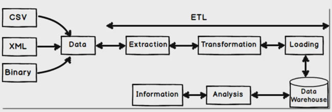
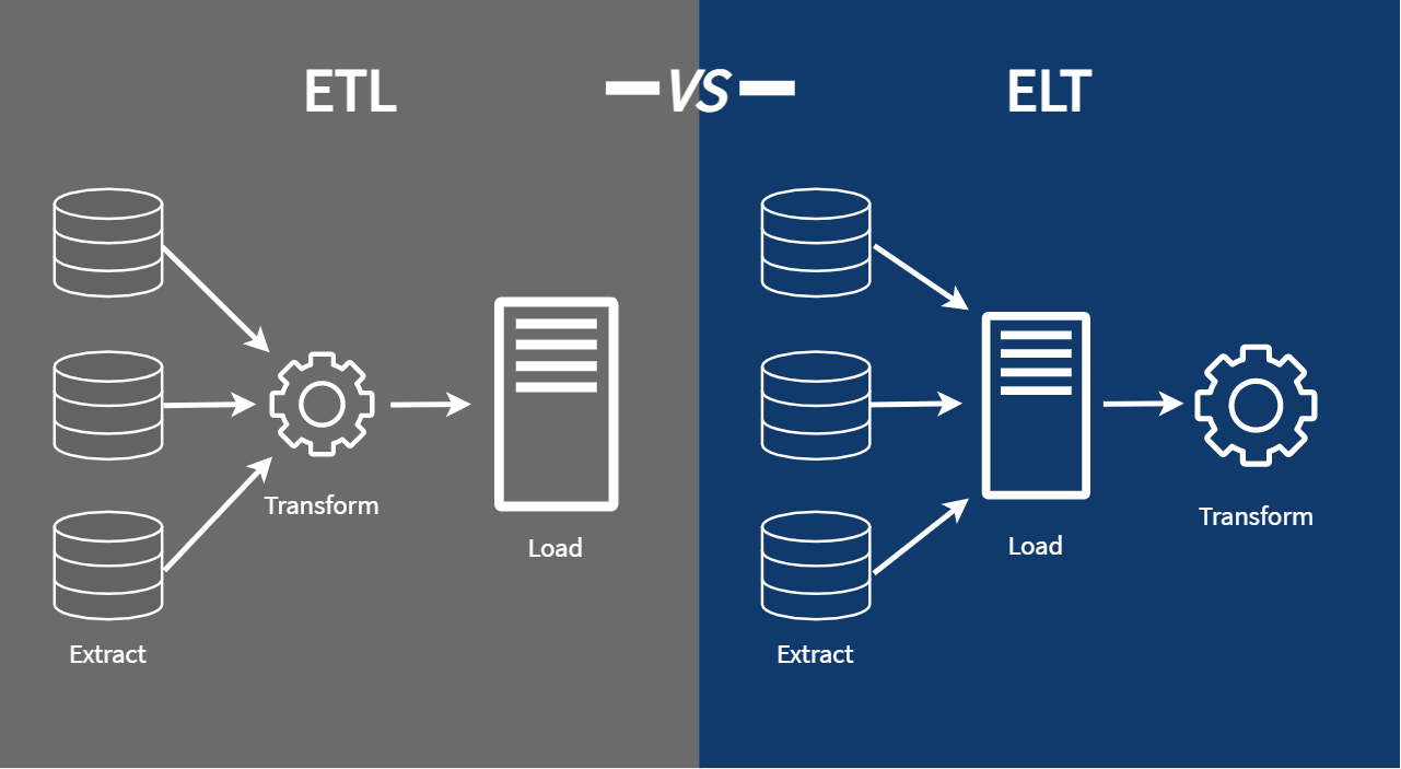
ETL: Extract Transform Load
ETL is a traditional data integration approach used primarily with RDBMS technologies such as MySQL, SQL Server, and Oracle.
Workflow
- Extract data from source systems.
- Transform it into the required format.
- Load it into the target system (e.g., a data warehouse).
ETL Tools
- SSIS / SSDT – SQL Server Integration Services / Data Tools
- Pentaho Kettle – Open-source ETL platform
- Talend – Data integration and transformation platform
- Benetl – Lightweight ETL for MySQL and PostgreSQL
ETL tools are well-suited for batch processing and structured environments but may struggle with scale and unstructured data.
src 1
src 2
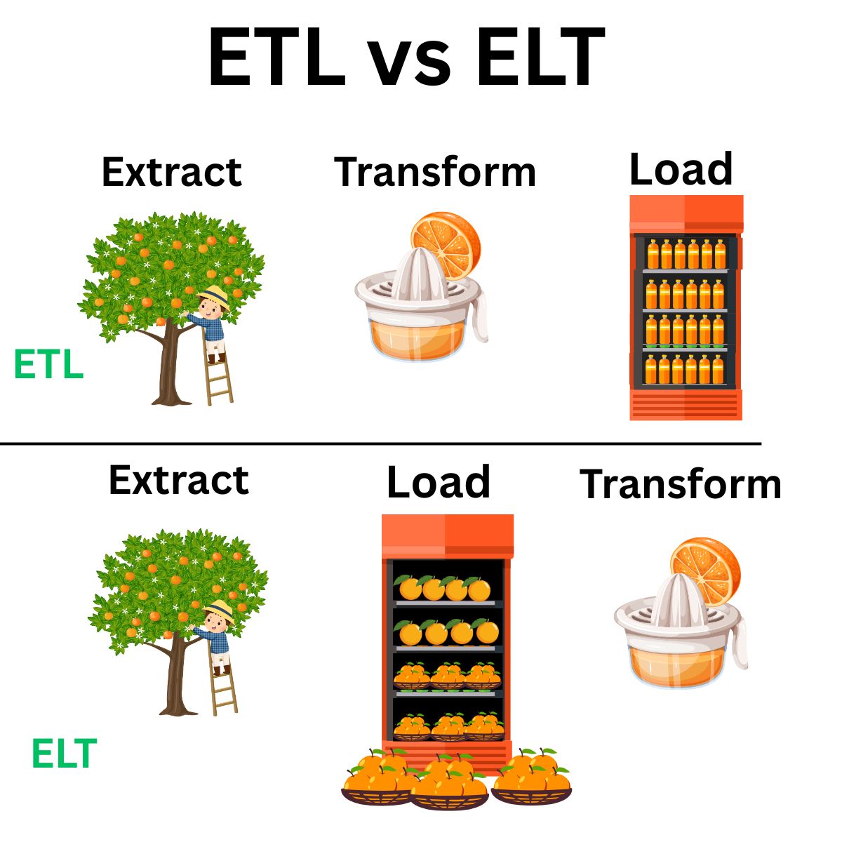
ELT: Extract Load Transform
ELT is the modern, Big Data-friendly approach. Instead of transforming data before loading, ELT prioritizes loading raw data first and transforming later.
Benefits
- Immediate ingestion of all types of data (structured or unstructured)
- Flexible transformation logic, applied post-load
- Faster load times and higher throughput
- Reduced operational overhead for loading processes
Challenges
- Security blind spots may arise from loading raw data upfront
- Compliance risks due to delayed transformation (HIPAA, GDPR, etc.)
- High storage costs if raw data is stored unfiltered in cloud/on-prem systems
ELT is ideal for data lakes, streaming, and cloud-native architectures.
Typical Big Data Flow
Raw Data → Cleansed Data → Data Processing → Data Warehousing → ML / BI / Analytics
- Raw Data: Initial unprocessed input (logs, JSON, CSV, APIs, sensors)
- Cleansed Data: Cleaned and standardized
- Processing: Performed through tools like Spark, DLT, or Flink
- Warehousing: Data is stored in structured formats (e.g., Delta, Parquet)
- Usage: Data is consumed by ML models, dashboards, or analysts
Each stage involves pipelines, validations, and metadata tracking.
#etl #elt #pipeline #rawdata #datalake
1: Leanmsbitutorial.com
2: https://towardsdatascience.com/how-i-redesigned-over-100-etl-into-elt-data-pipelines-c58d3a3cb3c
[Avg. reading time: 9 minutes]
Scaling & Distributed Systems
Scalability is a critical factor in Big Data and cloud computing. As workloads grow, systems must adapt.
There are two main ways to scale infrastructure:
vertical scaling and horizontal scaling. These often relate to how distributed systems are designed and deployed.
Vertical Scaling (Scaling Up)
Vertical scaling means increasing the capacity of a single machine.
Like upgrading your personal computer — adding more RAM, a faster CPU, or a bigger hard drive.
Pros:
- Simple to implement
- No code or architecture changes needed
- Good for monolithic or legacy applications
Cons:
- Hardware has physical limits
- Downtime may be required during upgrades
- More expensive hardware = diminishing returns
Used In:
- Traditional RDBMS
- Standalone servers
- Small-scale workloads
Horizontal Scaling (Scaling Out)
Horizontal scaling means adding more machines (nodes) to handle the load collectively.
Like hiring more team members instead of just working overtime yourself.
Pros:
- More scalable: Keep adding nodes as needed
- Fault tolerant: One machine failure doesn’t stop the system
- Supports distributed computing
Cons:
- More complex to configure and manage
- Requires load balancing, data partitioning, and synchronization
- More network overhead
Used In:
- Distributed databases (e.g., Cassandra, MongoDB)
- Big Data platforms (e.g., Hadoop, Spark)
- Cloud-native applications (e.g., Kubernetes)
Distributed Systems
A distributed system is a network of computers that work together to perform tasks. The goal is to increase performance, availability, and fault tolerance by sharing resources across machines.
Analogy:
A relay team where each runner (node) has a specific part of the race, but success depends on teamwork.
Key Features of Distributed Systems
| Feature | Description |
|---|---|
| Concurrency | Multiple components can operate at the same time independently |
| Scalability | Easily expand by adding more nodes |
| Fault Tolerance | If one node fails, others continue to operate with minimal disruption |
| Resource Sharing | Nodes share tasks, data, and workload efficiently |
| Decentralization | No single point of failure; avoids bottlenecks |
| Transparency | System hides its distributed nature from users (location, access, replication) |
Horizontal Scaling vs. Distributed Systems
| Aspect | Horizontal Scaling | Distributed System |
|---|---|---|
| Definition | Adding more machines (nodes) to handle workload | A system where multiple nodes work together as one unit |
| Goal | To increase capacity and performance by scaling out | To coordinate tasks, ensure fault tolerance, and share resources |
| Architecture | Not necessarily distributed | Always distributed |
| Coordination | May not require nodes to communicate | Requires tight coordination between nodes |
| Fault Tolerance | Depends on implementation | Built-in as a core feature |
| Example | Load-balanced web servers | Hadoop, Spark, Cassandra, Kafka |
| Storage/Processing | Each node may handle separate workloads | Nodes often share or split workloads and data |
| Use Case | Quick capacity boost (e.g., web servers) | Large-scale data processing, distributed storage |
Vertical scaling helps improve single-node power, while horizontal scaling enables distributed systems to grow flexibly. Most modern Big Data systems rely on horizontal scaling for scalability, reliability, and performance.
#scaling #vertical #horizontal #distributed
[Avg. reading time: 9 minutes]
CAP Theorem
 src 1
src 1
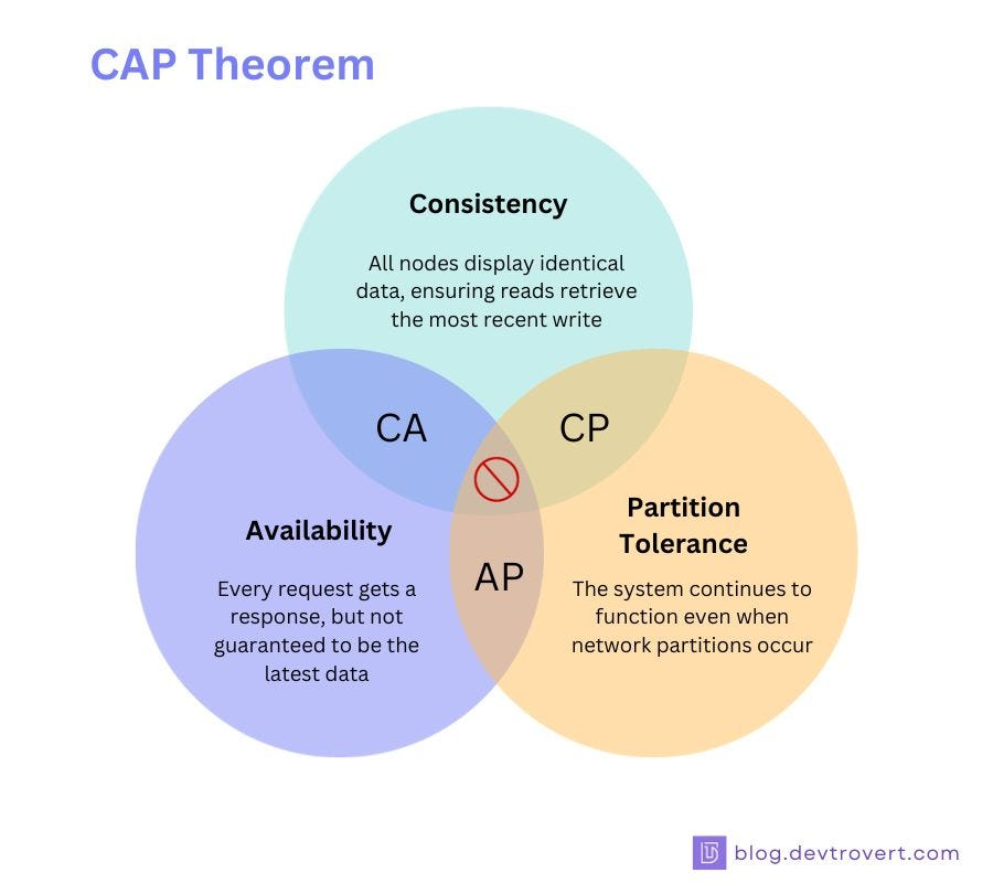
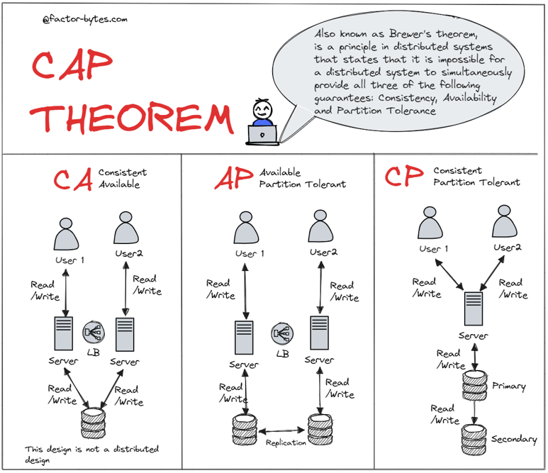
The CAP Theorem is a fundamental concept in distributed computing. It states that in the presence of a network partition, a distributed system can guarantee only two out of the following three properties:
The Three Components
-
Consistency (C)
Every read receives the most recent write or an error.
Example: If a book’s location is updated in a library system, everyone querying the catalog should see the updated location immediately. -
Availability (A)
Every request receives a (non-error) response, but not necessarily the most recent data.
Example: Like a convenience store that’s always open, even if they occasionally run out of your favorite snack. -
Partition Tolerance (P)
The system continues to function despite network failures or communication breakdowns.
Example: A distributed team in different rooms that still works, even if their intercom fails.
What the CAP Theorem Means
You can only pick two out of three:
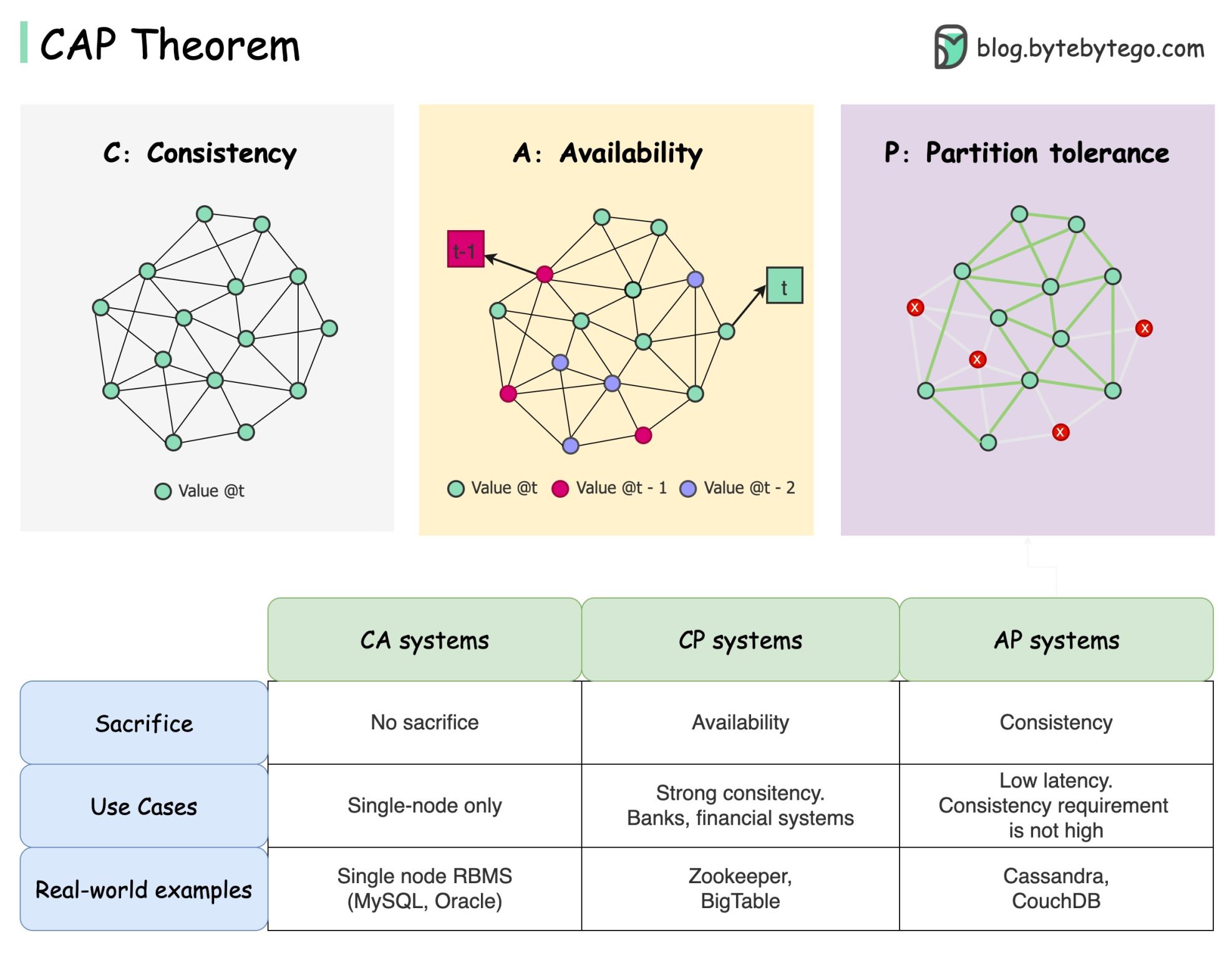
| Guarantee Combination | Sacrificed Property | Typical Use Case |
|---|---|---|
| CP (Consistency + Partition) | Availability | Banking Systems, RDBMS |
| AP (Availability + Partition) | Consistency | DNS, Web Caches |
| CA (Consistency + Availability) | Partition Tolerance (Not realistic in distributed systems) | Only feasible in non-distributed systems |
 src 2
src 2
Real-World Examples
CAP Theorem trade-offs can be seen in:
- Social Media Platforms – Favor availability and partition tolerance (AP)
- Financial Systems – Require consistency and partition tolerance (CP)
- IoT Networks – Often prioritize availability and partition tolerance (AP)
- eCommerce Platforms – Mix of AP and CP depending on the service
- Content Delivery Networks (CDNs) – Strongly AP-focused for high availability and responsiveness
 src 3
src 3
graph TD
    A[Consistency]
    B[Availability]
    C[Partition Tolerance]

    A -- CP System --> C
    B -- AP System --> C
    A -- CA System --> B

    subgraph CAP Triangle
        A
        B
        C
    end
This diagram shows that you can choose only two at a time:
- CP (Consistency + Partition Tolerance): e.g., traditional databases
- AP (Availability + Partition Tolerance): e.g., DNS, Cassandra
- CA is only theoretical in a distributed environment (it fails when partition occurs)
In distributed systems, network partitions are unavoidable. The CAP Theorem helps us choose which trade-off makes the most sense for our use case.
#cap #consistency #availability #partitiontolerant
1: blog.devtrovert.com
2: Factor-bytes.com
3: blog.bytebytego.com
[Avg. reading time: 6 minutes]
PACELC
The PACELC theorem is indeed a direct extension of the CAP theorem.
If Partition exists choose between Availability or Consistency Else Latency or Consistency
What If Partition Exists (P) means
- A network partition has occurred
- Some nodes cannot communicate with others
- Messages are dropped, not just delayed
When CAP exists why PACELC?
CAP focuses exclusively on what happens during a network failure (a “partition”), PACELC addresses a major critique: it accounts for how a system behaves during normal, healthy operation.
- Most systems run without network partitions most of the time
- Datacenters are engineered to avoid partitions
- Partitions are rare but catastrophic
- So when everything works, you still trade consistency vs latency.
                Distributed System
                        |
                        v
             Is there a network partition?
                        |
            +-----------+-----------+
            |                       |
          YES (P)                NO (ELSE)
            |                       |
            v                       v
   Availability (A)         Low Latency (L)
            |                       |
   - Keep serving            - Read nearest replica
   - May return              - Async replication
     inconsistent data       - Possible staleness
            |
            |
            v
     Consistency (C)         Consistency (C)
            |                       |
   - Block / error           - Quorum / consensus
   - Wait for quorum         - Higher latency
   - Data always correct     - Strong guarantees
| Database | P: Availability vs Consistency | ELSE: Latency vs Consistency | PACELC Class | Notes |
|---|---|---|---|---|
| Cassandra | Availability | Latency | PA / EL | Always-on design, async replication, eventual consistency |
| DynamoDB | Availability | Latency | PA / EL | Dynamo-style, low latency reads, consistency is optional |
| Riak | Availability | Latency | PA / EL | Conflict resolution after the fact |
| CouchDB | Availability | Latency | PA / EL | Multi-master replication, conflicts expected |
| MongoDB (Replica Set) | Consistency | Consistency | PC / EC | Primary-based writes, blocks during elections |
| HBase | Consistency | Consistency | PC / EC | Strong consistency via HDFS, higher coordination cost |
| Google Spanner | Consistency | Consistency | PC / EC | Global consensus, correctness over latency |
| CockroachDB | Consistency | Consistency | PC / EC | Distributed SQL, serializable isolation |
| Elasticsearch | Availability | Latency | PA / EL | Search-first, stale reads acceptable |
| Redis Cluster | Availability | Latency | PA / EL | Speed first, eventual consistency under failure |
[Avg. reading time: 6 minutes]
Optimistic concurrency
Optimistic Concurrency is a concurrency control strategy used in databases and distributed systems that allows multiple users or processes to access the same data simultaneously—without locking resources.
Instead of preventing conflicts upfront by using locks, it assumes that conflicts are rare. If a conflict does occur, it’s detected after the operation, and appropriate resolution steps (like retries) are taken.
How It Works
- Multiple users/processes read and attempt to write to the same data.
- Instead of using locks, each update tracks the version or timestamp of the data.
- When writing, the system checks if the data has changed since it was read.
- If no conflict, the write proceeds.
- If conflict detected, the system throws an exception or prompts a retry.
Let’s look at a simple example:
Sample inventory Table
| item_id | item_nm | stock |
|---------|---------|-------|
|    1    | Apple   |  10   |
|    2    | Orange  |  20   |
|    3    | Banana  |  30   |
Imagine two users, UserA and UserB, trying to update the apple stock simultaneously.
User A’s update:
UPDATE inventory SET stock = stock + 5 WHERE item_id = 1;
User B’s update:
UPDATE inventory SET stock = stock - 3 WHERE item_id = 1;
- Both updates execute concurrently without locking the table.
- After both operations, system checks for version conflicts.
- If there’s no conflict, the changes are merged.
New price of Apple stock = 10 + 5 - 3 = 12
- If there was a conflicting update (e.g., both changed the same field from different base versions), one update would fail, and the user must retry the transaction.
Optimistic Concurrency Is Ideal When
| Condition | Explanation |
|---|---|
| Low write contention | Most updates happen on different parts of data |
| Read-heavy, write-light systems | Updates are infrequent or less overlapping |
| High performance is critical | Avoiding locks reduces wait times |
| Distributed systems | Locking is expensive and hard to coordinate |
[Avg. reading time: 6 minutes]
Eventual consistency
Eventual consistency is a consistency model used in distributed systems (like NoSQL databases and distributed storage) where updates to data may not be immediately visible across all nodes. However, the system guarantees that all replicas will eventually converge to the same state — given no new updates are made.
Unlike stronger models like serializability or linearizability, eventual consistency prioritizes performance and availability, especially in the face of network latency or partitioning.
Simple Example: Distributed Key-Value Store
Imagine a distributed database with three nodes: Node A, Node B, and Node C. All store the value for a key called "item_stock":
Node A: item_stock = 10
Node B: item_stock = 10
Node C: item_stock = 10
Now, a user sends an update to change item_stock to 15, and it reaches only Node A initially:
Node A: item_stock = 15
Node B: item_stock = 10
Node C: item_stock = 10
At this point, the system is temporarily inconsistent. Over time, the update propagates:
Node A: item_stock = 15
Node B: item_stock = 15
Node C: item_stock = 10
Eventually, all nodes reach the same value:
Node A: item_stock = 15
Node B: item_stock = 15
Node C: item_stock = 15
Key Characteristics
- Temporary inconsistencies are allowed
- Data will converge across replicas over time
- Reads may return stale data during convergence
- Prioritizes availability and partition tolerance over strict consistency
When to Use Eventual Consistency
Eventual consistency is ideal when:
| Situation | Why It Helps |
|---|---|
| High-throughput, low-latency systems | Avoids the overhead of strict consistency |
| Geo-distributed deployments | Tolerates network delays and partitions |
| Systems with frequent writes | Enables faster response without locking or blocking |
| Availability is more critical than accuracy | Keeps services running even during network issues |
[Avg. reading time: 6 minutes]
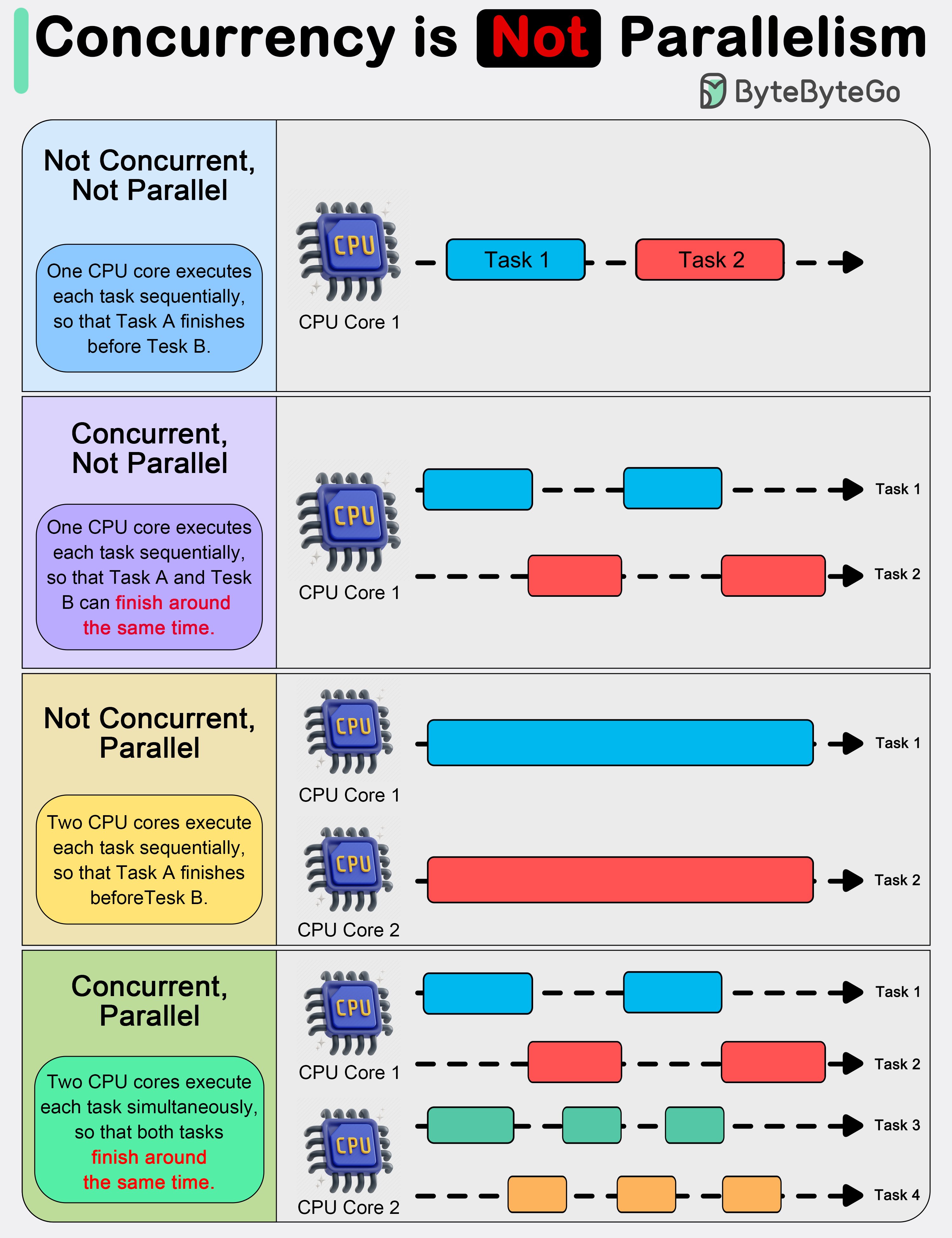
Concurrent vs. Parallel
Understanding the difference between concurrent and parallel programming is key when designing efficient, scalable applications — especially in distributed and multi-core systems.
Concurrent Programming
Concurrent programming is about managing multiple tasks at once, allowing them to make progress without necessarily executing at the same time.
- Tasks overlap in time.
- Focuses on task coordination, not simultaneous execution.
- Often used in systems that need to handle many events or users, like web servers or GUIs.
Key Traits
- Enables responsive programs (non-blocking)
- Utilizes a single core or limited resources efficiently
- Requires mechanisms like threads, coroutines, or async/await
Parallel Programming
Parallel programming is about executing multiple tasks simultaneously, typically to speed up computation.
- Tasks run at the same time, often on multiple cores.
- Focuses on performance and efficiency.
- Common in high-performance computing, such as scientific simulations or data processing.
Key Traits
- Requires multi-core CPUs or GPUs
- Ideal for data-heavy workloads
- Uses multithreading, multiprocessing, or vectorization
Analogy: Cooking in a Kitchen
Concurrent Programming
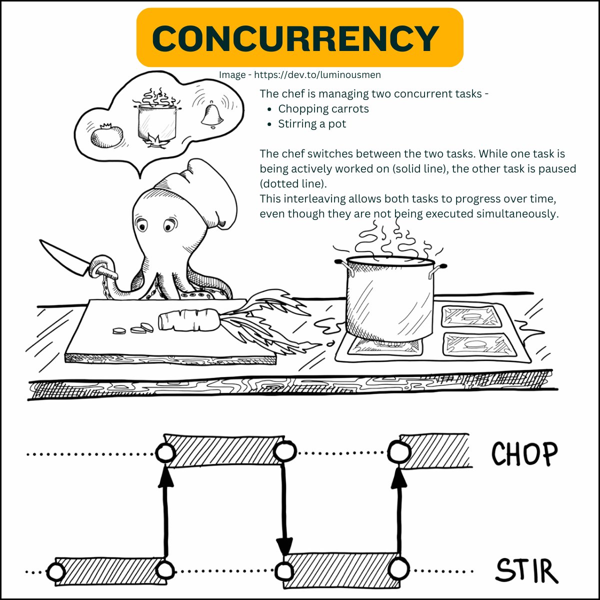
One chef is working on multiple dishes. While a pot is simmering, the chef chops vegetables for the next dish. Tasks overlap, but only one is actively running at a time.
Parallel Programming
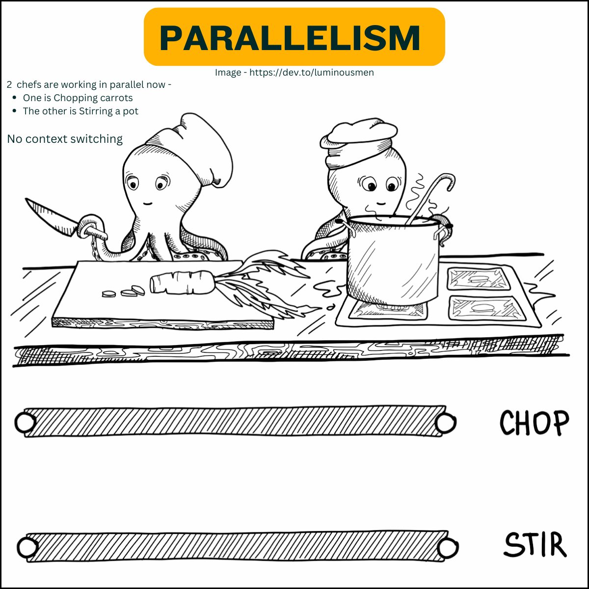
A team of chefs in a large kitchen, each cooking a different dish at the same time. Multiple dishes are actively being cooked simultaneously, speeding up the overall process.
Summary Table
| Feature | Concurrent Programming | Parallel Programming |
|---|---|---|
| Task Timing | Tasks overlap, but not necessarily at once | Tasks run simultaneously |
| Focus | Managing multiple tasks efficiently | Improving performance through parallelism |
| Execution Context | Often single-core or logical thread | Multi-core, multi-threaded or GPU-based |
| Tools/Mechanisms | Threads, coroutines, async I/O | Threads, multiprocessing, SIMD, OpenMP |
| Example Use Case | Web servers, I/O-bound systems | Scientific computing, big data, simulations |
#concurrent #parallelprogramming
[Avg. reading time: 3 minutes]
General-Purpose Language (GPL)
What is a GPL?
A GPL is a programming language designed to write software in multiple problem domains. It is not limited to a particular application area.
Swiss Army Knife

Examples
- Python – widely used in ML, web, scripting, automation.
- Java – enterprise applications, Android, backend.
- C++ – system programming, game engines.
- Rust – performance + memory safety.
- JavaScript – web front-end & server-side with Node.js.
Use Cases
- Building web apps (backend/frontend).
- Developing AI/ML pipelines.
- Writing system software and operating systems.
- Implementing data processing frameworks (e.g., Apache Spark in Scala).
- Creating mobile and desktop applications.
Why Use GPL?
- Flexibility to work across domains.
- Rich standard libraries and ecosystems.
- Ability to combine different kinds of tasks (e.g., networking + ML).
[Avg. reading time: 4 minutes]
DSL
A DSL is a programming or specification language dedicated to a particular problem domain, a particular problem representation technique, and/or a particular solution technique.
Examples
- SQL – querying and manipulating relational databases.
- HTML – for structuring content on the web.
- R – statistical computing and graphics.
- Makefiles – for building projects.
- Regular Expressions – for pattern matching.
- Markdown (READ.md or https://stackedit.io/app#)
- Mermaid - Mermaid (https://mermaid.live/)
Use Cases
- Building data pipelines (e.g., dbt, Airflow DAGs).
- Writing infrastructure-as-code (e.g., Terraform HCL).
- Designing UI layout (e.g., QML for Qt UI design).
- IoT rule engines (e.g., IFTTT or Node-RED flows).
- Statistical models using R.
Why Use DSL?
- Shorter, more expressive code in the domain.
- Higher-level abstractions.
- Reduced risk of bugs for domain experts.
Optional Challenge: Build Your Own DSL!
Design your own mini Domain-Specific Language (DSL)! You can keep it simple.
- Start with a specific problem.
- Create your own syntax that feels natural to all.
- Try few examples and ask your friends to try.
- Try implementing a parser using your favourite GPL.
[Avg. reading time: 4 minutes]
Popular Big Data Tools & Platforms
Big Data ecosystems rely on a wide range of tools and platforms for data processing, real-time analytics, streaming, and cloud-scale storage. Here’s a list of some widely used tools categorized by functionality:
Distributed Processing Engines
- Apache Spark – Unified analytics engine for large-scale data processing; supports batch, streaming, and ML.
- Apache Flink – Framework for stateful computations over data streams with real-time capabilities.
Real-Time Data Streaming
- Apache Kafka – Distributed event streaming platform for building real-time data pipelines and streaming apps.
Log & Monitoring Stack
- ELK Stack (Elasticsearch, Logstash, Kibana) – Searchable logging and visualization suite for real-time analytics.
Cloud-Based Platforms
- AWS (Amazon Web Services) – Scalable cloud platform offering Big Data tools like EMR, Redshift, Kinesis, and S3.
- Azure – Microsoft’s cloud platform with tools like Azure Synapse, Data Lake, and Event Hubs.
- GCP (Google Cloud Platform) – Offers BigQuery, Dataflow, Pub/Sub for large-scale data analytics.
- Databricks – Unified data platform built around Apache Spark with powerful collaboration and ML features.
- Snowflake – Cloud-native data warehouse known for performance, elasticity, and simplicity.
#bigdata #tools #cloud #kafka #spark
[Avg. reading time: 3 minutes]
NoSQL Database Types
NoSQL databases are optimized for flexibility, scalability, and performance, making them ideal for Big Data and real-time applications. They are categorized based on how they store and access data:
Key-Value Stores
Store data as simple key-value pairs. Ideal for caching, session storage, and high-speed lookups.
- Redis
- Amazon DynamoDB
Columnar Stores
Store data in columns rather than rows, optimized for analytical queries and large-scale batch processing.
- Apache HBase
- Apache Cassandra
- Amazon Redshift
Document Stores
Store semi-structured data like JSON or BSON documents. Great for flexible schemas and content management systems.
- MongoDB
- Amazon DocumentDB
Graph Databases
Use nodes and edges to represent and traverse relationships between data. Ideal for social networks, recommendation engines, and fraud detection.
- Neo4j
- Amazon Neptune
Tip: Choose the NoSQL database type based on your data access patterns and application needs.
Not all NoSQL databases solve the same problem.
#nosql #keyvalue #documentdb #graphdb #columnar
[Avg. reading time: 4 minutes]
Learning Big Data
Learning Big Data goes beyond just handling large datasets. It involves building a foundational understanding of data types, file formats, processing tools, and cloud platforms used to store, transform, and analyze data at scale.
Types of Files & Formats
- Data File Types: CSV, JSON
- File Formats: CSV, TSV, TXT, Parquet
Linux & File Management Skills
- Essential Linux Commands:
ls,cat,grep,awk,sort,cut,sed, etc. - Useful Libraries & Tools:
awk,jq,csvkit,grep– for filtering, transforming, and managing structured data
Data Manipulation Foundations
- Regular Expressions: For pattern matching and advanced string operations
- SQL / RDBMS: Understanding relational data and query languages
- NoSQL Databases: Working with document, key-value, columnar, and graph stores
Cloud Technologies
- Introduction to major platforms: AWS, Azure, GCP
- Services for data storage, compute, and analytics (e.g., S3, EMR, BigQuery)
Big Data Tools & Frameworks
- Tools like Apache Spark, Flink, Kafka, Dask
- Workflow orchestration (e.g., Airflow, DBT, Databricks Workflows)
Miscellaneous Tools & Libraries
- Visualization:
matplotlib,seaborn,Plotly - Data Engineering:
pandas,pyarrow,sqlalchemy - Streaming & Real-time:
Kafka,Spark Streaming,Flume
Tip: Big Data learning is a multi-disciplinary journey. Start small — explore files and formats — then gradually move into tools, pipelines, cloud platforms, and real-time systems.
[Avg. reading time: 0 minutes]
Developer Tools
[Avg. reading time: 5 minutes]
Introduction
Before diving into Data or ML frameworks, it's important to have a clean and reproducible development setup. A good environment makes you:
- Faster: less time fighting dependencies.
- Consistent: same results across laptops, servers, and teammates.
- Confident: tools catch errors before they become bugs.
A consistent developer experience saves hours of debugging. You spend more time solving problems, less time fixing environments.
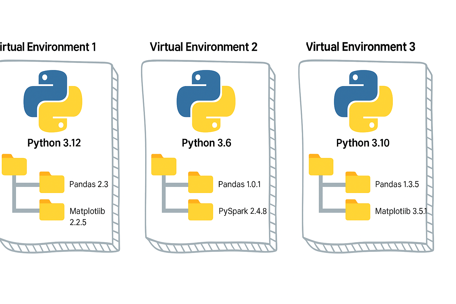
Python Virtual Environment
- A virtual environment is like a sandbox for Python.
- It isolates your project’s dependencies from the global Python installation.
- Easy to manage different versions of library.
- Must depend on requirements.txt, it has to be managed manually.
Without it, installing one package for one project may break another project.
#venv #python #uv #poetry developer_tools
[Avg. reading time: 3 minutes]
UV
Dependency & Environment Manager
- Written in Rust.
- Syntax is lightweight.
- Automatic Virtual environment creation.
Create a new project:
# Initialize a new uv project
uv init uv_helloworld
Sample layout of the directory structure
.
├── main.py
├── pyproject.toml
├── README.md
└── uv.lock
# Change directory
cd uv_helloworld

# # Create a virtual environment myproject
# uv venv myproject

# or create a UV project with specific version of Python

# uv venv myproject --python 3.11

# # Activate the Virtual environment

# source myproject/bin/activate

# # Verify the Virtual Python version

# which python3

# add library (best practice)
uv add faker

# verify the list of libraries under virtual env
uv tree

# To find the list of libraries inside Virtual env

uv pip list
edit the main.py
from faker import Faker
fake = Faker()
print(fake.name())
uv run main.py
Read More on the differences between UV and Poetry
[Avg. reading time: 17 minutes]
Python Developer Tools
PEP
PEP, or Python Enhancement Proposal, is the official style guide for Python code. It provides conventions and recommendations for writing readable, consistent, and maintainable Python code.
- PEP 8 : Style guide for Python code (most famous).
- PEP 20 : "The Zen of Python" (guiding principles).
- PEP 484 : Type hints (basis for MyPy).
- PEP 517/518 : Build system interfaces (basis for pyproject.toml, used by Poetry/UV).
- PEP 572 : Assignment expressions (the := walrus operator).
- PEP 440 : Mention versions in Libraries
PEP 8 (Popular one)
Indentation
- Use 4 spaces per indentation level
- Continuation lines should align with opening delimiter or be indented by 4 spaces.
Line Length
- Limit lines to a maximum of 79 characters.
- For docstrings and comments, limit lines to 72 characters.
Blank Lines
- Use 2 blank lines before top-level functions and class definitions.
- Use 1 blank line between methods inside a class.
Imports
- Imports should be on separate lines.
- Group imports into three sections: standard library, third-party libraries, and local application imports.
- Use absolute imports whenever possible.
# Correct
    import os
    import sys

# Wrong
    import sys, os
Naming Conventions
- Use
snake_casefor function and variable names. - Use
CamelCasefor class names. - Use
UPPER_SNAKE_CASEfor constants. - Avoid single-character variable names except for counters or indices.
Whitespace
- Don’t pad inside parentheses/brackets/braces.
- Use one space around operators and after commas, but not before commas.
- No extra spaces when aligning assignments.
Comments
- Write comments that are clear, concise, and helpful.
- Use complete sentences and capitalize the first word.
- Use # for inline comments, but avoid them where the code is self-explanatory.
Docstrings
- Use triple quotes (""") for multiline docstrings.
- Describe the purpose, arguments, and return values of functions and methods.
Code Layout
- Keep function definitions and calls readable.
- Avoid writing too many nested blocks.
Consistency
- Consistency within a project outweighs strict adherence.
- If you must diverge, be internally consistent.
PEP 20 - The Zen of Python
https://peps.python.org/pep-0020/
Simple is better than complex
Complex
result = (lambda x: (x*x + 2*x + 1))(5)
Simple
x = 5
result = (x + 1) ** 2
Readability counts
No Good
a=10;b=20;c=a+b;print(c)
Good
first_value = 10
second_value = 20
sum_of_values = first_value + second_value
print(sum_of_values)
Errors should never pass silently
No Good
try:
    x = int("abc")
except:
    pass
Good
try:
    x = int("abc")
except ValueError as e:
    print("Conversion failed:", e)
PEP 572
Walrus Operator :=
Assignment within Expression Operator
Old Way
inputs = []
current = input("Write something ('quit' to stop): ")
while current != "quit":
    inputs.append(current)
    current = input("Write something ('quit' to stop): ")
Using Walrus
inputs = []
while (current := input("Write something ('quit' to stop): ")) != "quit":
    inputs.append(current)
Another Example
Old Way
import re

m = re.search(r"\d+", text)
if m:
    print(m.group())
New Way
import re

if (m := re.search(r"\d+", text)):
    print(m.group())
Linting
Linting is the process of automatically checking your Python code for:
-
Syntax errors
-
Stylistic issues (PEP 8 violations)
-
Potential bugs or bad practices
-
Keeps your code consistent and readable.
-
Helps catch errors early before runtime.
-
Encourages team-wide coding standards.
# Incorrect
import sys, os

# Correct
import os
import sys
# Bad spacing
x= 5+3

# Good spacing
x = 5 + 3
Ruff : Linter and Code Formatter
Ruff is a fast, modern tool written in Rust that helps keep your Python code:
- Consistent (follows PEP 8)
- Clean (removes unused imports, fixes spacing, etc.)
- Correct (catches potential errors)
Install
uv add ruff
Verify
ruff --version
ruff --help
example.py
import os, sys

def greet(name):
  print(f"Hello, {name}")

def message(name): print(f"Hi, {name}")

def calc_sum(a, b): return a+b

greet('World')
greet('Ruff')
message('Ruff')
uv run ruff check example.py
uv run ruff check example.py --fix
uv run ruff format example.py --check
uv run ruff check example.py
PEP 484 - MyPy : Type Checking Tool
Python is a Dynamically typed programming language. Meaning
x=26 x= "hello"
both are valid.
MyPy is introduced to make it statically typed.
mypy is a static type checker for Python. It checks your code against the type hints you provide, ensuring that the types are consistent throughout the codebase.
It primarily focuses on type correctness—verifying that variables, function arguments, return types, and expressions match the expected types.
What mypy checks:
- Variable reassignment types
- Function arguments
- Return types
- Expressions and operations
- Control flow narrowing
What mypy does not do:
- Runtime validation
- Performance checks
- Logical correctness
Install
    uv add mypy

    or

    pip install mypy
Example 1 : sample.py
x = 1
x = 1.0
x = True
x = "test"
x = b"test"

print(x)
uv run mypy sample.py

or

mypy sample.py
Example 2: Type Safety
def add(a: int, b: int) -> int:
    return a + b

print(add(100, 123))
print(add("hello", "world"))
Example 3: Return Type Violation
def divide(a: int, b: int) -> int:
    if b == 0:
        return "invalid"
    return a // b
Example 4: Optional Types
from typing import Optional

def get_username(user_id: int) -> Optional[str]:
    if user_id == 0:
        return None
    return "admin"

name = get_username(0)
print(name.upper())
What is wrong in this? name can also be None and there is no upper for None
[Avg. reading time: 0 minutes]
Dataformat
[Avg. reading time: 6 minutes]
Introduction to Data Formats
What Are Data Formats?
- Data formats define how data is represented on disk or over the wire
- They describe:
- Structure (rows, columns, trees, blocks)
- Encoding (text, binary)
- Schema handling (strict, flexible, embedded, external)
- In Big Data, data formats are not just a storage choice, they are a performance decision
Why Data Formats Matter in Big Data
- Big Data systems deal with:
- Huge volumes
- Distributed storage
- Parallel processing
- A poor format choice can:
- Waste storage
- Slow down queries by orders of magnitude
- Break downstream systems
Choosing the right format directly impacts:
- Storage efficiency
- Scan speed
- Compression ratio
- CPU usage
- Network I/O
This is why data engineers care about formats more than application developers do.
Big Data Reality Check
- Data rarely lives in a single database
- Data moves through:
- APIs
- Message queues
- Object storage
- Data lakes
- File formats become the contract between systems
Once data is written in a format, changing it later is expensive.
Data Formats vs Traditional Database Storage
| Feature | Traditional RDBMS | Big Data Formats |
|---|---|---|
| Storage Unit | Tables | Files or streams |
| Schema | Fixed, enforced on write | Often flexible or schema-on-read |
| Access Pattern | Row-based | Row, column, or block-based |
| Optimization | Indexes, transactions | Partitioning, compression, vectorized reads |
| Scale Model | Vertical or limited horizontal | Designed for distributed systems |
| Typical Use | OLTP, dashboards | ETL, analytics, ML pipelines |
Key Shift for Data Engineers
- Databases optimize queries
- Data formats optimize data movement and scanning
- In Big Data:
- Data is written once
- Read many times
- Often by different engines
That’s why formats like CSV, JSON, Avro, Parquet, and ORC exist, each solving a different problem.
What This Chapter Will Cover
- Text vs binary formats
- Row-based vs columnar storage
- Schema-on-write vs schema-on-read
- When formats break at scale
- Why Parquet dominates analytics workloads
[Avg. reading time: 3 minutes]
Common Data Formats
CSV (Comma-Separated Values)
A simple text-based format where each row represents a record and each column is separated by a comma.
Example
name,age,city
Rachel,30,New York
Phoebe,25,San Francisco
Use Cases
- Data exchange between systems
- Lightweight storage
- Import/export from databases and spreadsheets
Pros
- Human-readable
- Easy to generate and parse
- Supported by almost every tool
Cons
- No support for nested or complex structures
- No schema enforcement
- No data types, everything is text
- Inefficient for very large datasets
TSV (Tab-Separated Values)
Similar to CSV, but uses tab characters instead of commas as delimiters.
Example
name    age    city
Rachel   30     New York
Phoebe     25     San Francisco
Use Cases
- Same use cases as CSV
- Useful when data contains commas frequently
Pros
- Simple and human-readable
- Avoids issues with commas inside values
- Easy to parse
Cons
- No schema enforcement
- No nested or complex data support
- Same scalability and performance issues as CSV
#bigdata #dataformat #csv #tsv
[Avg. reading time: 6 minutes]
JSON
JavaScript Object Notation
- Neither row-based nor columnar
- Flexible way to store and share data across systems
- Text-based format using curly braces and key-value pairs
Simplest JSON Example
{"id": "1","name":"Rachel"}
Properties
- Language independent
- Self-describing
- Human-readable
- Widely supported across platforms
Basic Rules
- Curly braces
{}hold objects - Data is represented as key-value pairs
- Entries are separated by commas
- Double quotes are mandatory
- Square brackets
[]hold arrays
JSON Values
String  {"name":"Rachel"}

Number  {"id":101}

Boolean {"result":true, "status":false}  (lowercase)

Object  {
            "character":{"fname":"Rachel","lname":"Green"}
        }

Array   {
            "characters":["Rachel","Ross","Joey","Chanlder"]
        }

NULL    {"id":null}
Sample JSON Document
{
    "characters": [
        {
            "id" : 1,
            "fName":"Rachel",
            "lName":"Green",
            "status":true
        },
        {
            "id" : 2,
            "fName":"Ross",
            "lName":"Geller",
            "status":true
        },
        {
            "id" : 3,
            "fName":"Chandler",
            "lName":"Bing",
            "status":true
        },
        {
            "id" : 4,
            "fName":"Phebe",
            "lName":"Buffay",
            "status":false
        }
    ]
}
JSON Best Practices
No Hyphen in your Keys.
{"first-name":"Rachel","last-name":"Green"} is not right. ✘
data.first-name
is parsed as
(data.first) - (name)
Under Scores Okay
{"first_name":"Rachel","last_name":"Green"} is okay ✓
Lowercase Okay
{"firstname":"Rachel","lastname":"Green"} is okay ✓
Camelcase best
{"firstName":"Rachel","lastName":"Green"} is the best. ✓
Use Cases
- APIs and web services
- Configuration files
- NoSQL databases
- Serialization and deserialization
Python Example
Serialize : Convert Python Object to JSON (Shareable) Format. DeSerialize : Convert JSON (Shareable) String to Python Object.
import json

def json_serialize(file_name):
    friends_characters={
        "characters":[
            {"name":"Rachel Green","job":"Fashion Executive"},
            {"name":"Ross Geller","job":"Paleontologist"},
            {"name":"Monica Geller","job":"Chef"},
            {"name":"Chandler Bing","job":"Statistical Analysis and Data Reconfiguration"},
            {"name":"Joey Tribbiani","job":"Actor"},
            {"name":"Phoebe Buffay","job":"Massage Therapist"}
        ]
    }
    json_data=json.dumps(friends_characters,indent=4)
    with open(file_name,"w") as f:
        json.dump(friends_characters,f,indent=4)

def json_deserialize(file_name):
    with open(file_name,"r") as f:
        data=json.load(f)
    print(data,type(data))

def main():
    file_name="friends_characters.json"
    json_serialize(file_name)
    json_deserialize(file_name)

if __name__=="__main__":
    main()
#bigdata #dataformat #json #hierarchical
[Avg. reading time: 16 minutes]
Parquet
Parquet is a columnar storage file format designed for big data analytics.
- Optimized for reading large datasets
- Works extremely well with engines like Spark, Hive, DuckDB, Athena
- Best suited for WORM workloads (Write Once, Read Many)
Why Parquet Exists
Most analytics questions look like this:
- Total sales per country
- Total T-Shirts sold
- Revenue for UK customers
These queries do not need all columns.
Row-based formats still scan everything.
Parquet does not.
Row-Based Storage (CSV, JSON)
If you ask:
Total T-Shirts sold or Customers from UK
The engine must scan every column of every row.
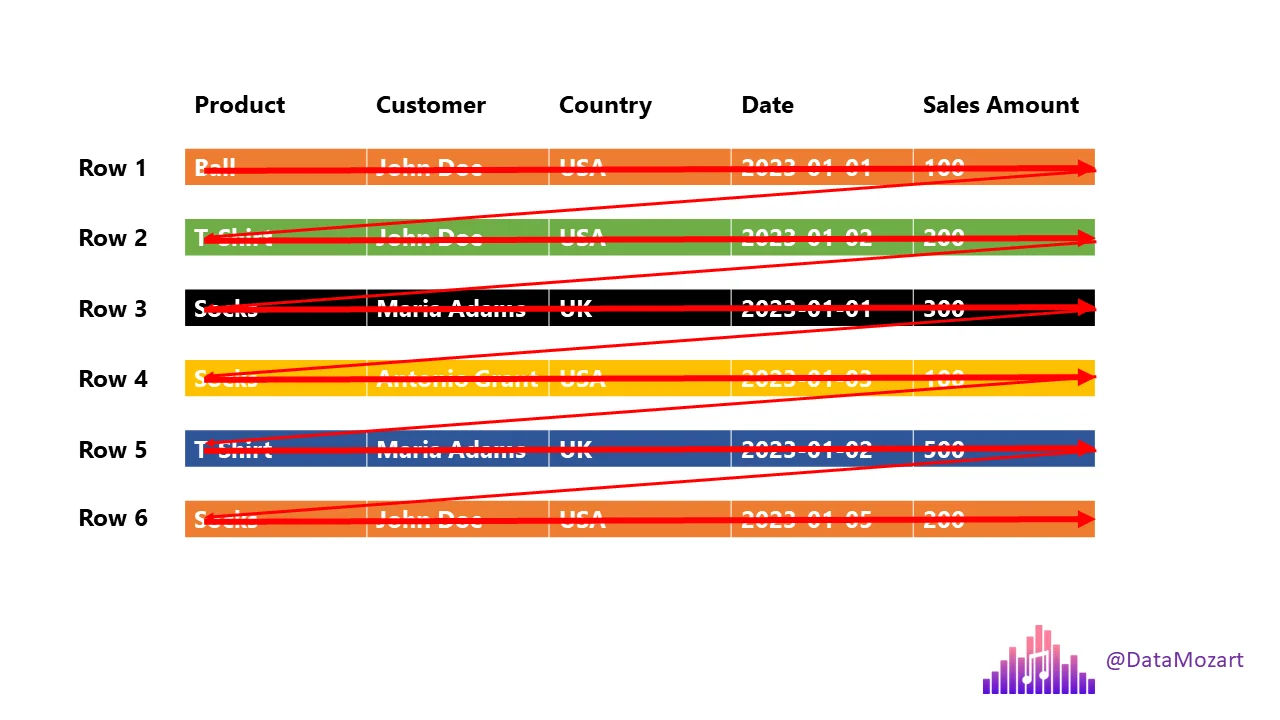
This is slow at scale.
Columnar Storage (Parquet)
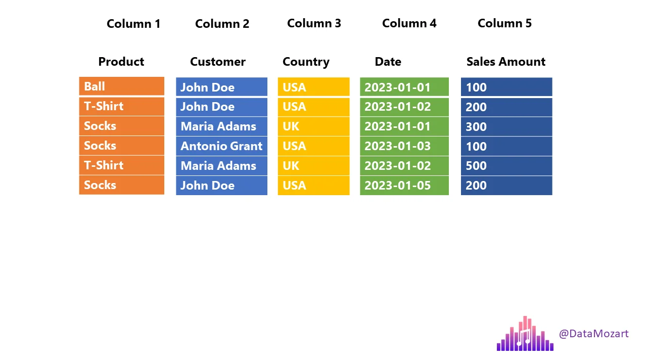
- Each column is stored separately
- Queries read only required columns
- Massive reduction in disk I/O
Two Important Query Terms
Projection
Columns required by the query.
select product, country, salesamount from sales;
Projection:
- product
- country
- salesamount
Predicate
Row-level filter condition.
select product, country, salesamount from sales where country='UK';
Predicate:
country = 'UK'
Parquet uses metadata to skip unnecessary data.
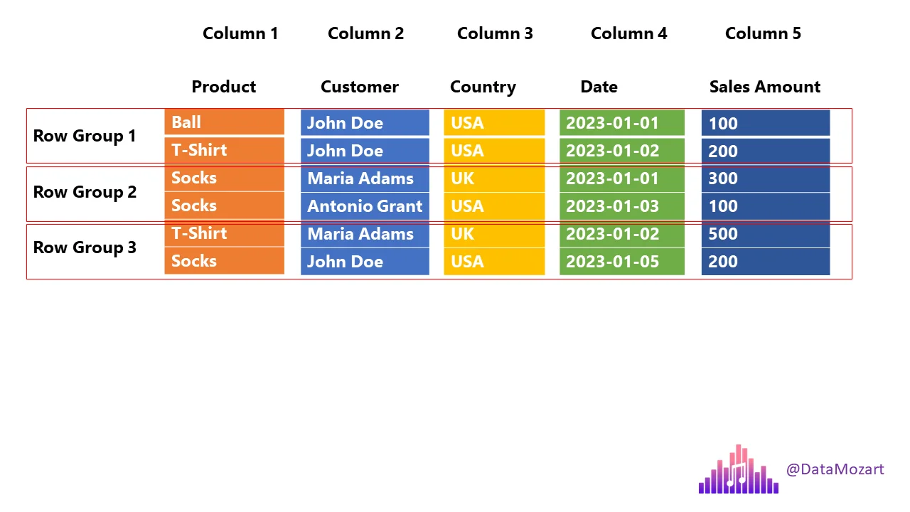
Row Groups
Parquet splits data into row groups.
Each row group contains:
- All columns
- Metadata (min/max values)
This allows:
- Parallel processing
- Skipping row groups that don’t match filters.
Parquet - Columnar Storage + Row Groups
Sample Data
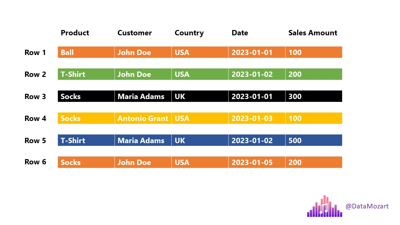
| Product | Customer | Country | Date | Sales Amount |
|---|---|---|---|---|
| Ball | John Doe | USA | 2023-01-01 | 100 |
| T-Shirt | John Doe | USA | 2023-01-02 | 200 |
| Socks | Jane Doe | UK | 2023-01-03 | 150 |
| Socks | Jane Doe | UK | 2023-01-04 | 180 |
| T-Shirt | Alex | USA | 2023-01-05 | 120 |
| Socks | Alex | USA | 2023-01-06 | 220 |
Data stored inside Parquet
┌──────────────────────────────────────────────┐
│                File Header                   │
│  ┌────────────────────────────────────────┐  │
│  │ Magic Number: "PAR1"                   │  │
│  └────────────────────────────────────────┘  │
├──────────────────────────────────────────────┤
│                Row Group 1                   │
│  ┌────────────────────────────────────────┐  │
│  │ Column Chunk: Product                  │  │
│  │  ├─ Page 1: Ball, T-Shirt, Socks       │  │
│  └────────────────────────────────────────┘  │
│  ┌────────────────────────────────────────┐  │
│  │ Column Chunk: Customer                 │  │
│  │  ├─ Page 1: John Doe, John Doe, Jane Doe│ │
│  └────────────────────────────────────────┘  │
│  ┌────────────────────────────────────────┐  │
│  │ Column Chunk: Country                  │  │
│  │  ├─ Page 1: USA, USA, UK               │  │
│  └────────────────────────────────────────┘  │
│  ┌────────────────────────────────────────┐  │
│  │ Column Chunk: Date                     │  │
│  │  ├─ Page 1: 2023-01-01, 2023-01-02,    │  │
│  │            2023-01-03                  │  │
│  └────────────────────────────────────────┘  │
│  ┌────────────────────────────────────────┐  │
│  │ Column Chunk: Sales Amount             │  │
│  │  ├─ Page 1: 100, 200, 150              │  │
│  └────────────────────────────────────────┘  │
│  ┌────────────────────────────────────────┐  │
│  │ Row Group Metadata                     │  │
│  │  ├─ Num Rows: 3                        │  │
│  │  ├─ Min/Max per Column:                │  │
│  │     • Product: Ball/T-Shirt/Socks      │  │
│  │     • Customer: Jane Doe/John Doe      │  │
│  │     • Country: UK/USA                  │  │
│  │     • Date: 2023-01-01 to 2023-01-03    │  │
│  │     • Sales Amount: 100 to 200         │  │
│  └────────────────────────────────────────┘  │
├──────────────────────────────────────────────┤
│                Row Group 2                   │
│  ┌────────────────────────────────────────┐  │
│  │ Column Chunk: Product                  │  │
│  │  ├─ Page 1: Socks, T-Shirt, Socks      │  │
│  └────────────────────────────────────────┘  │
│  ┌────────────────────────────────────────┐  │
│  │ Column Chunk: Customer                 │  │
│  │  ├─ Page 1: Jane Doe, Alex, Alex       │  │
│  └────────────────────────────────────────┘  │
│  ┌────────────────────────────────────────┐  │
│  │ Column Chunk: Country                  │  │
│  │  ├─ Page 1: UK, USA, USA               │  │
│  └────────────────────────────────────────┘  │
│  ┌────────────────────────────────────────┐  │
│  │ Column Chunk: Date                     │  │
│  │  ├─ Page 1: 2023-01-04, 2023-01-05,    │  │
│  │            2023-01-06                  │  │
│  └────────────────────────────────────────┘  │
│  ┌────────────────────────────────────────┐  │
│  │ Column Chunk: Sales Amount             │  │
│  │  ├─ Page 1: 180, 120, 220              │  │
│  └────────────────────────────────────────┘  │
│  ┌────────────────────────────────────────┐  │
│  │ Row Group Metadata                     │  │
│  │  ├─ Num Rows: 3                        │  │
│  │  ├─ Min/Max per Column:                │  │
│  │     • Product: Socks/T-Shirt           │  │
│  │     • Customer: Alex/Jane Doe          │  │
│  │     • Country: UK/USA                  │  │
│  │     • Date: 2023-01-04 to 2023-01-06   │  │
│  │     • Sales Amount: 120 to 220         │  │
│  └────────────────────────────────────────┘  │
├──────────────────────────────────────────────┤
│                File Metadata                 │
│  ┌────────────────────────────────────────┐  │
│  │ Schema:                                │  │
│  │  • Product: string                     │  │
│  │  • Customer: string                    │  │
│  │  • Country: string                     │  │
│  │  • Date: date                          │  │
│  │  • Sales Amount: double                │  │
│  ├────────────────────────────────────────┤  │
│  │ Compression Codec: Snappy              │  │
│  ├────────────────────────────────────────┤  │
│  │ Num Row Groups: 2                      │  │
│  ├────────────────────────────────────────┤  │
│  │ Offsets to Row Groups                  │  │
│  │  • Row Group 1: offset 128             │  │
│  │  • Row Group 2: offset 1024            │  │
│  └────────────────────────────────────────┘  │
├──────────────────────────────────────────────┤
│                File Footer                   │
│  ┌────────────────────────────────────────┐  │
│  │ Offset to File Metadata: 2048          │  │
│  │ Magic Number: "PAR1"                   │  │
│  └────────────────────────────────────────┘  │
└──────────────────────────────────────────────┘
Example:
SELECT product, salesamount
FROM sales
WHERE country = 'UK';
Parquet will:
- Read only product, salesamount, country
- Skip row groups where country != UK
- Ignore all other columns
This is why Parquet is fast.
Compression
Parquet compresses per column, which works very well.
Common codecs:
Snappy
- Fast
- Low CPU usage
- Lower compression
- Used in hot / frequently queried data
GZip
- Slower
- Higher compression
- Used in cold / archival data
Encoding
Encoding reduces storage before compression.
Dictionary Encoding
- Replaces repeated values with small integers
- 0: Ball
- 1: T-Shirt
- 2: Socks
- Data Page: [0,1,2,2,1,2]
Run-Length Encoding
- Compresses repeated consecutive values
If Country column was sorted: [USA, USA, USA, UK, UK, UK]
RLE: [(3, USA), (3, UK)]
Delta Encoding
- Stores differences between values (dates, counters)
This makes Parquet compact and efficient.
Date column: [2023-01-01, 2023-01-02, 2023-01-03, ...]
Delta Encoding: [2023-01-01, +1, +1, +1, ...]
Summary about Parquet
- Columnar storage
- Very fast analytical queries
- Excellent compression
- Schema support
- Works across languages and engines
- Industry standard for data lakes
Python Example
import pandas as pd

file_path = 'https://raw.githubusercontent.com/gchandra10/filestorage/main/sales_100.csv'

# Read the CSV file
df = pd.read_csv(file_path)

# Display the first few rows of the DataFrame
print(df.head())

# Write DataFrame to a Parquet file
df.to_parquet('sample.parquet')
Some utilities to inspect Parquet files
WIN/MAC
https://aloneguid.github.io/parquet-dotnet/parquet-floor.html#installing
MAC
https://github.com/hangxie/parquet-tools
parquet-tools row-count sample.parquet
parquet-tools schema sample.parquet
parquet-tools cat sample.parquet
parquet-tools meta sample.parquet
Remote Files
parquet-tools row-count https://github.com/gchandra10/filestorage/raw/refs/heads/main/sales_onemillion.parquet
#bigdata #dataformat #parquet #columnar #compressed
[Avg. reading time: 9 minutes]
Apache Arrow
Apache Arrow is an in-memory columnar data format designed for fast data exchange and analytics.
- Parquet is for disk
- Arrow is for memory
Arrow allows different systems to share data without copying or converting it.
Why Arrow Exists
Traditional formats focus on storage:
- CSV, JSON → human-readable, slow
- Parquet → compressed, efficient on disk
But once data is loaded into memory:
- Engines still spend time converting data
- Python, JVM, C++, R all use different memory layouts
Arrow solves this by providing a common in-memory columnar layout.
What Arrow Is Good At
- Fast in-memory analytics
- Zero-copy data sharing
- Cross-language interoperability
- Vectorized processing
Arrow is not a replacement for Parquet.
They work together.
Row-by-Row vs Vectorized Processing
Row-wise Processing (Slow)
Each value is processed one at a time.
data=[1,2,3,4]
for i in range(len(data)):
    data[i]=data[i]+10
Vectorized Processing (Fast)
One operation runs on the entire column at once.
import numpy as np
data=np.array([1,2,3,4])
data=data+10
Zero-Copy
Normally:
- Data is copied when moving between tools
- Copying costs time and memory
With Arrow:
- Arrow enables zero-copy of Data when systems support it.
- No serialization.
- No extra copies.
Parquet → Arrow → Pandas → ML → Arrow → Parquet
- Fast, clean, efficient.
| Feature | Apache Arrow | Apache Parquet |
|---|---|---|
| Purpose | In-memory analytics | On-disk storage |
| Location | RAM | Disk |
| Performance | Very fast, interactive | Optimized for scans |
| Compression | Minimal | Heavy compression |
| Use Case | Data exchange, compute | Data lakes, warehousing |
Demonstration (With and Without Vectorization)
import time
import numpy as np
import pyarrow as pa

N = 10_000_000
data_list = list(range(N))           # Python list
data_array = np.arange(N)            # NumPy array
arrow_arr = pa.array(data_list)      # Arrow array
np_from_arrow = arrow_arr.to_numpy() # Convert Arrow buffer to NumPy

# ---- Traditional Python list loop ----
start = time.time()
result1 = [x + 1 for x in data_list]
print(f"List processing time: {time.time() - start:.4f} seconds")

# ---- NumPy vectorized ----
start = time.time()
result2 = data_array + 1
print(f"NumPy processing time: {time.time() - start:.4f} seconds")

# ---- Arrow + NumPy ----
start = time.time()
result3 = np_from_arrow + 1
print(f"Arrow + NumPy processing time: {time.time() - start:.4f} seconds")
Use Cases
Data Science & Machine Learning
- Share data between Pandas, Spark, R, and ML libraries without copying or converting.
Streaming & Real-Time Analytics
- Ideal for passing large datasets through streaming frameworks with low latency.
Data Exchange
- Move data between different systems with a common representation (e.g. Pandas → Spark → R).
Big Data
- Integrates with Parquet, Avro, and other formats for ETL and analytics.
Think of Arrow as the in-memory twin of Parquet: Arrow is perfect for fast, interactive analytics; Parquet is great for long-term, compressed storage.
[Avg. reading time: 5 minutes]
Avro
Avro is a row-based binary data serialization format designed for data exchange and streaming systems.
Unlike Parquet, Avro is optimized for writing and reading one record at a time.
Why Avro Exists
Many systems need to:
- Send data between producers and consumers
- Handle continuous streams of events
- Evolve data schemas safely over time
Text formats like JSON are:
- Easy to read
- Slow and verbose
Avro solves this with:
- Compact binary encoding
- Strong schema support
Key Characteristics
- Row-based format
- Supports Schema evolution
- Binary and compact
- Schema-driven
- Designed for interoperability
- Excellent for streaming pipelines
Schema in Avro
Avro uses a JSON schema to define data structure.
The schema:
- Describes fields and data types
- Travels with the data or is shared separately
- Enables backward and forward compatibility
Example schema:
{
  "type": "record",
  "name": "Person",
  "fields": [
    {"name": "firstName", "type": "string"},
    {"name": "lastName", "type": "string"},
    {"name": "age", "type": "int"},
    {"name": "email", "type": ["null","string"], "default": null}
  ]
}
Where Avro Is Used
- Kafka producers and consumers
- Streaming and real-time pipelines
- Data ingestion layers
- Cross-language data exchange
When NOT to Use Avro
- Analytical queries
- Aggregations
- Column-level filtering
Avro vs Parquet
| Feature | Avro | Parquet |
|---|---|---|
| Storage Style | Row-based | Columnar |
| Optimized For | Streaming, writes | Analytics, reads |
| Typical Access | One record at a time | Selected columns |
| Compression | Moderate | Very high |
| Common Use | Kafka, ingestion | Data lakes, OLAP |
tags:dataformat #avro #rowbased
[Avg. reading time: 4 minutes]
YAML
YAML stands for YAML Ain’t Markup Language.
- Human-readable data serialization format
- Designed for configuration, not large datasets
- Structure is defined by indentation
- Whitespace matters
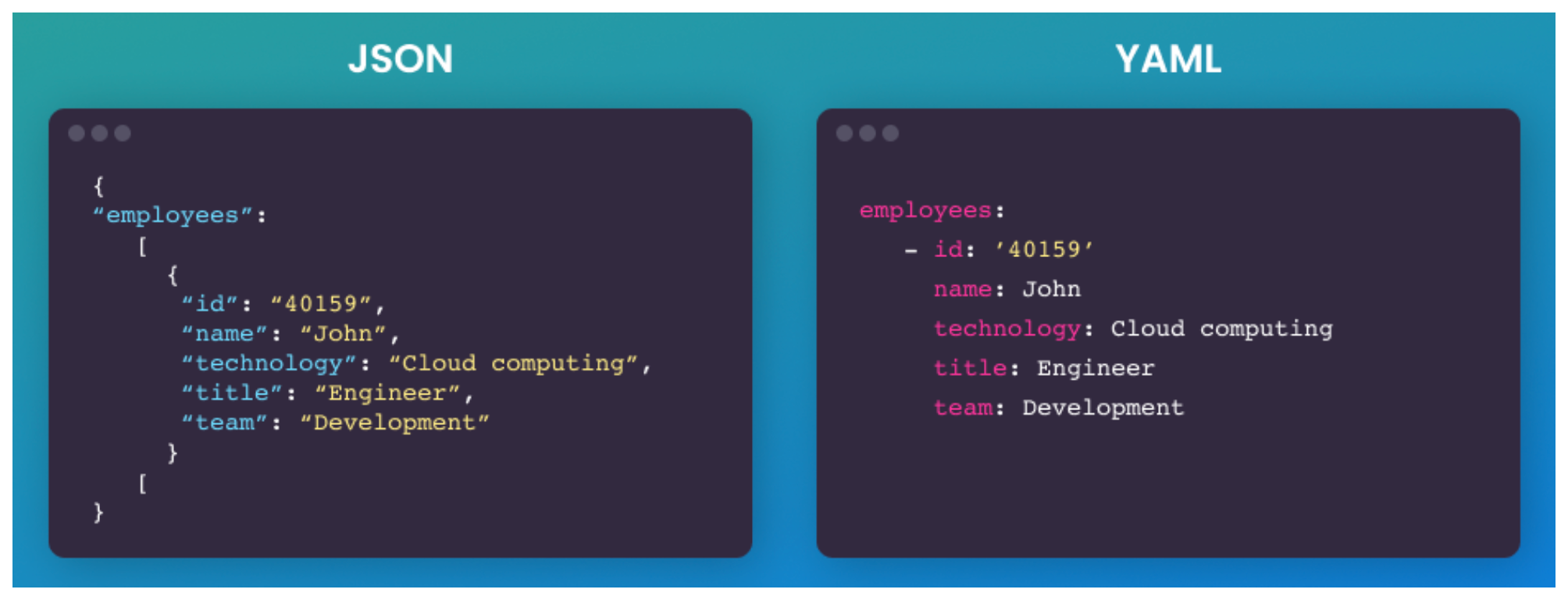
Core Data Structures
Key–Value (Map / Dictionary)
app: analytics
version: 1.0
List (Sequence / Array)
ports:
  - 8080
  - 9090
Nested structures
database:
  host: localhost
  port: 5432
  credentials:
    user: admin
    password: secret
Scalars
- string, int, float, bool, null
- true, false, null are native types
YAML vs JSON
- YAML is superet of JSON, YAML can parse JSON syntax.
- No braces, no commas
- Comments are allowed
- Types inferred, not enforced
- Easier diffs in git
- Easier to break with bad indentation
Tradeoff is real. YAML is readable but fragile.
{"id":1,"name":"event","tags":["click","mobile"]}
id: 1
name: event
tags:
  - click
  - mobile
Real world usecases
Here are some of the popular usecases in Data Engineering
- CICD
- Terraform
- Docker
- Airflow
JSON is for DATA and YAML is for Config
YAML is a bad choice for Data if
- Dataset is Large
- High Write frequency
- Streaming or Continous Data
- Schema critical systems
Because
- YAML is slow to parse (compared to JSON)
- Hard to validate strictly
- No native indexing
- YAML parsers build large memory trees
Lightweight portable command-line
https://mikefarah.gitbook.io/yq/
[Avg. reading time: 9 minutes]
DuckDB
DuckDB is a lightweight analytical database designed to run locally with no external dependencies.
- Single-file database
- Zero setup
- Optimized for analytics
- Excellent support for modern data formats like Parquet
DuckDB is often called the SQLite for analytics.
Why DuckDB Is Useful Here
DuckDB helps us experience the impact of data formats.
It allows us to:
- Query CSV and Parquet directly
- See why columnar formats are faster
- Run analytical queries without Spark or a cluster
DuckDB is a tool for learning, not the topic itself.
Key Capabilities (High Level)
- Automatic parallel query execution
- Fast analytical SQL engine
- Native Parquet support
- Reads files directly without loading them into tables
- Works well with Python and data science workflows
Download the CLI Client
-
Linux).
-
For other programming languages, visit https://duckdb.org/docs/installation/
-
Unzip the file.
-
Open Command / Terminal and run the Executable.
DuckDB in Data Engineering
Download orders.parquet
Open Command Prompt or Terminal
./duckdb

or

duckdb.exe
# Create / Open a database

.open ordersdb
Duckdb allows you to read the contents of orders.parquet as is without needing a table. Double quotes around the file name orders.parquet is essential.
describe table "orders.parquet"
select * from "orders.parquet" limit 3;
show tables;

create table orders  as select * from "orders.parquet";

select count(*) from orders;
DuckDB supports parallel query processing, and queries run fast.
This table has 1.5 million rows, and aggregation happens in less than a second.
select now(); select o_orderpriority,count(*) cnt from orders group by o_orderpriority; select now();
DuckDB also helps to convert parquet files to CSV in a snap. It also supports converting CSV to Parquet.
COPY "orders.parquet" to 'orders.csv' (FORMAT "CSV", HEADER 1);Select * from "orders.csv" limit 3;
It also supports exporting existing Tables to Parquet files.
COPY "orders" to 'neworder.parquet' (FORMAT "PARQUET");
DuckDB supports Programming languages such as Python, R, JAVA, node.js, C/C++.
DuckDB ably supports Higher-level SQL programming such as Macros, Sequences, Window Functions.
Get sample data from Yellow Cab
https://www.nyc.gov/site/tlc/about/tlc-trip-record-data.page
Copy yellow cabs data into yellowcabs folder
create table taxi_trips as select * from "yellowcabs/*.parquet";
SELECT
    PULocationID,
    EXTRACT(HOUR FROM tpep_pickup_datetime) AS hour_of_day,
    AVG(fare_amount) AS avg_fare
FROM
    taxi_trips
GROUP BY
    PULocationID,
    hour_of_day;
Extensions
https://duckdb.org/docs/extensions/overview
INSTALL json;
LOAD json;
select * from demo.json;
describe demo.json;
Load directly from HTTP location
select * from 'https://raw.githubusercontent.com/gchandra10/filestorage/main/sales_100.csv'
#duckdb #singlefiledatabase #parquet #tools #cli
[Avg. reading time: 1 minute]
Protocols
- Introduction
- HTTP
- Monolithic Architecture
- Statefulness
- Microservices
- Statelessness
- Idempotency
- REST API
- API Performance
- API in Big Data world
[Avg. reading time: 2 minutes]
Introduction
Protocols are standardized rules that govern how data is transmitted, formatted, and processed across systems.
In Big Data, protocols are essential for:
- Data ingestion (getting data in)
- Inter-node communication in clusters
- Remote access to APIs/services
- Serialization of structured data
- Security and authorization
| Protocol | Layer | Use Case Example |
|---|---|---|
| HTTP/HTTPS | Application | REST API for ingesting external data |
| Kafka | Messaging | Stream processing with Spark or Flink |
| gRPC | RPC | Microservices in ML model serving |
| MQTT | Messaging | IoT data push to cloud |
| Avro/Proto | Serialization | Binary data for logs and schema |
| OAuth/Kerberos | Security | Secure access to data lakes |
[Avg. reading time: 2 minutes]
HTTP
Basics
HTTP (HyperText Transfer Protocol) is the foundation of data communication on the web, used to transfer data (such as HTML files and images).
GET - Navigate to a URL or click a link in real life.
POST - Submit a form on a website, like a username and password.
Popular HTTP Status Codes
200 Series (Success): 200 OK, 201 Created.
300 Series (Redirection): 301 Moved Permanently, 302 Found.
400 Series (Client Error): 400 Bad Request, 401 Unauthorized, 404 Not Found.
500 Series (Server Error): 500 Internal Server Error, 503 Service Unavailable.
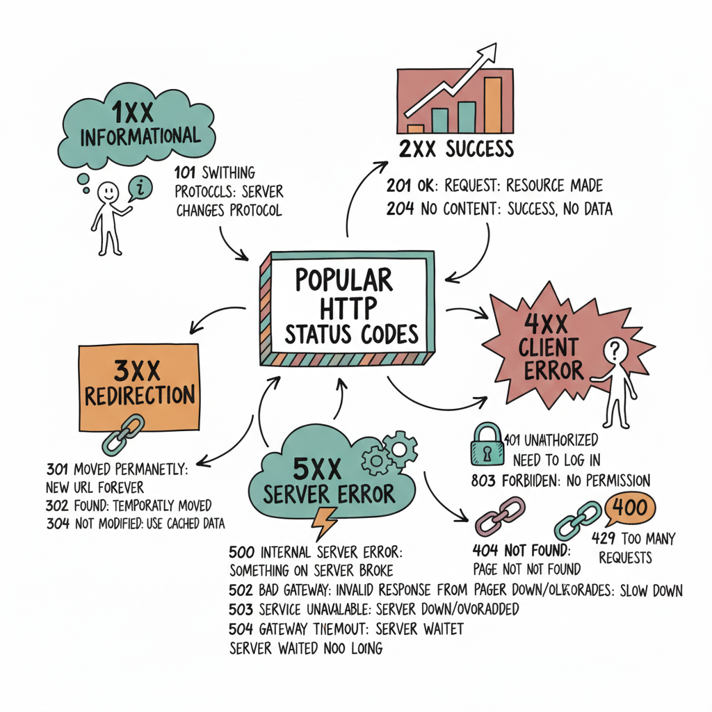
#http #get #put #post #statuscodes
[Avg. reading time: 3 minutes]
Monolithic Architecture
Definition: A monolithic architecture is a software design pattern in which an application is built as a unified unit. All application components (user interface, business logic, and data access layers) are tightly coupled and run as a single service.
Characteristics: This architecture is simple to develop, test, deploy, and scale vertically. However, it can become complex and unwieldy as the application grows.

Examples
- Traditional Banking Systems.
- Enterprise Resource Planning (SAP ERP) Systems.
- Content Management Systems like WordPress.
- Legacy Government Systems. (Tax filing, public records management, etc.)
Advantages and Disadvantages
Advantages: Simplicity in development and deployment, straightforward horizontal scaling, and often more accessible debugging since all components are in one place. Reduced Latency in the case of Amazon Prime.
Disadvantages: Scaling challenges, difficulty implementing changes or updates (especially in large systems), and potential for more extended downtime during maintenance.
#monolithic #banking #amazonprime tightlycoupled
[Avg. reading time: 8 minutes]
Statefulness
The server stores information about the client’s current session in a stateful system. This is common in traditional web applications. Here’s what characterizes a stateful system:
Session Memory: The server remembers past interactions and may store session data like user authentication, preferences, and other activities.
Server Dependency: Since the server holds session data, the same server usually handles subsequent requests from the same client. This is important for consistency.
Resource Intensive: Maintaining state can be resource-intensive, as the server needs to manage and store session data for each client.
Example: A web application where a user logs in, and the server keeps track of their authentication status and interactions until they log out.
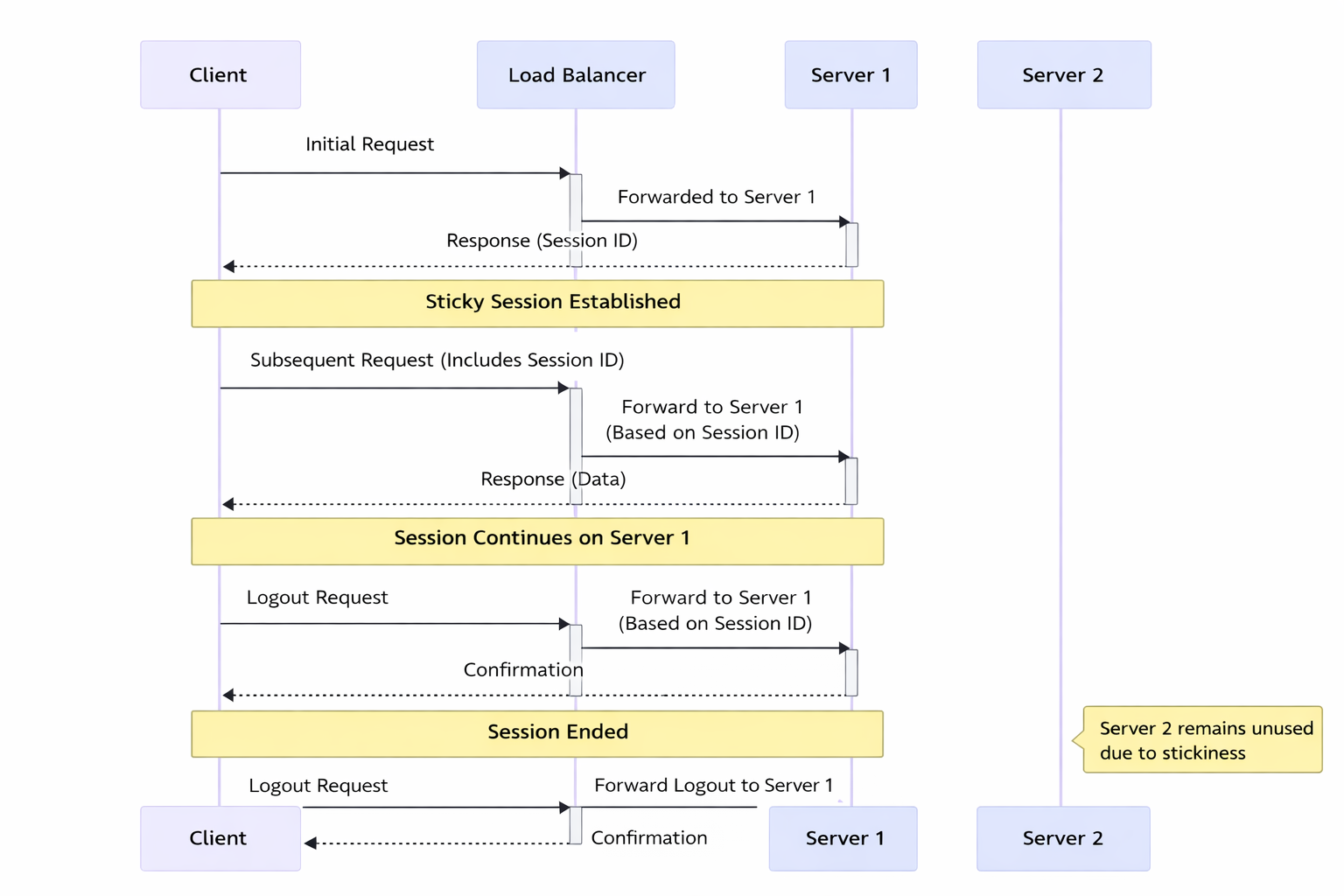
In this diagram:
Initial Request: The client sends the initial request to the load balancer.
Load Balancer to Server 1: The load balancer forwards the request to Server 1.
Response with Session ID: Server 1 responds to the client with a session ID, establishing a sticky session.
Subsequent Requests: The client sends subsequent requests with the session ID.
Load Balancer Routes to Server 1: The load balancer forwards these requests to Server 1 based on the session ID, maintaining the sticky session.
Server 1 Processes Requests: Server 1 continues to handle requests from this client.
Server 2 Unused: Server 2 remains unused for this particular client due to the stickiness of the session with Server 1.
Stickiness (Sticky Sessions)
Stickiness or sticky sessions are used in stateful systems, particularly in load-balanced environments. It ensures that requests from a particular client are directed to the same server instance. This is important when:
Session Data: The server needs to maintain session data (like login status), and it’s stored locally on a specific server instance.
Load Balancers: In a load-balanced environment, without stickiness, a client’s requests could be routed to different servers, which might not have the client’s session data.
Trade-off: While it helps maintain session continuity, it can reduce the load balancing efficiency and might lead to uneven server load.
Methods of Implementing Stickiness
Cookie-Based Stickiness: The most common method, where the load balancer uses a special cookie to track the server assigned to a client.
IP-Based Stickiness: The load balancer routes requests based on the client’s IP address, sending requests from the same IP to the same server.
Custom Header or Parameter: Some load balancers can use custom headers or URL parameters to track and maintain session stickiness.
#stateful #stickiness #loadbalancer
[Avg. reading time: 9 minutes]
Microservices
Microservices architecture is a method of developing software applications as a suite of small, independently deployable services. Each service in a microservices architecture is focused on a specific business capability, runs in its process, and communicates with other services through well-defined APIs. This approach stands in contrast to the traditional monolithic architecture, where all components of an application are tightly coupled and run as a single service.
Characteristics:
Modularity: The application is divided into smaller, manageable pieces (services), each responsible for a specific function or business capability.
Independence: Each microservice is independently deployable, scalable, and updatable. This allows for faster development cycles and easier maintenance.
Decentralized Control: Microservices promote decentralized data management and governance. Each service manages its data and logic.
Technology Diversity: Teams can choose the best technology stack for their microservice, leading to a heterogeneous technology environment.
Resilience: Failure in one microservice doesn’t necessarily bring down the entire application, enhancing the system’s overall resilience.
Scalability: Microservices can be scaled independently, allowing for more efficient resource utilization based on demand for specific application functions.
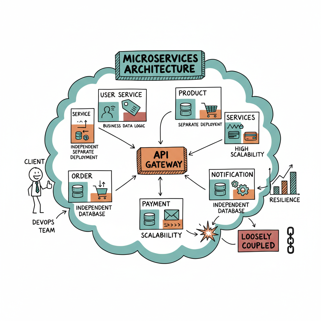
Data Ingestion Microservices: Collect and process data from multiple sources.
Data Storage: Stores processed weather data and other relevant information.
User Authentication Microservice: Manages user authentication and communicates with the User Database for validation.
User Database: Stores user account information and preferences.
API Gateway: Central entry point for API requests, routes requests to appropriate microservices, and handles user authentication.
User Interface Microservice: Handles the logic for the user interface, serving web and mobile applications.
Data Retrieval Microservice: Fetches weather data from the Data Storage and provides it to the frontends.
Web Frontend: The web interface for end-users, making requests through the API Gateway.
Mobile App Backend: Backend services for the mobile application, also making requests through the API Gateway.
Advantages:
Agility and Speed: Smaller codebases and independent deployment cycles lead to quicker development and faster time-to-market.
Scalability: It is easier to scale specific application parts that require more resources.
Resilience: Isolated services reduce the risk of system-wide failures.
Flexibility in Technology Choices: Microservices can use different programming languages, databases, and software environments.
Disadvantages:
Complexity: Managing a system of many different services can be complex, especially regarding network communication, data consistency, and service discovery.
Overhead: Each microservice might need its own database and transaction management, leading to duplication and increased resource usage.
Testing Challenges: Testing inter-service interactions can be more complex compared to a monolithic architecture.
Deployment Challenges: Requires robust DevOps practices, including continuous integration and continuous deployment (CI/CD) pipelines.
[Avg. reading time: 6 minutes]
Statelessness
In a stateless system, each request from the client must contain all the information the server needs to fulfill that request. The server does not store any state of the client’s session. This is a crucial principle of RESTful APIs. Characteristics include:
No Session Memory: The server remembers nothing about the user once the transaction ends. Each request is independent.
Scalability: Stateless systems are generally more scalable because the server doesn’t need to maintain session information. Any server can handle any request.
Simplicity and Reliability: The stateless nature makes the system simpler and more reliable, as there’s less information to manage and synchronize across systems.
Example: An API where each request contains an authentication token and all necessary data, allowing any server instance to handle any request.
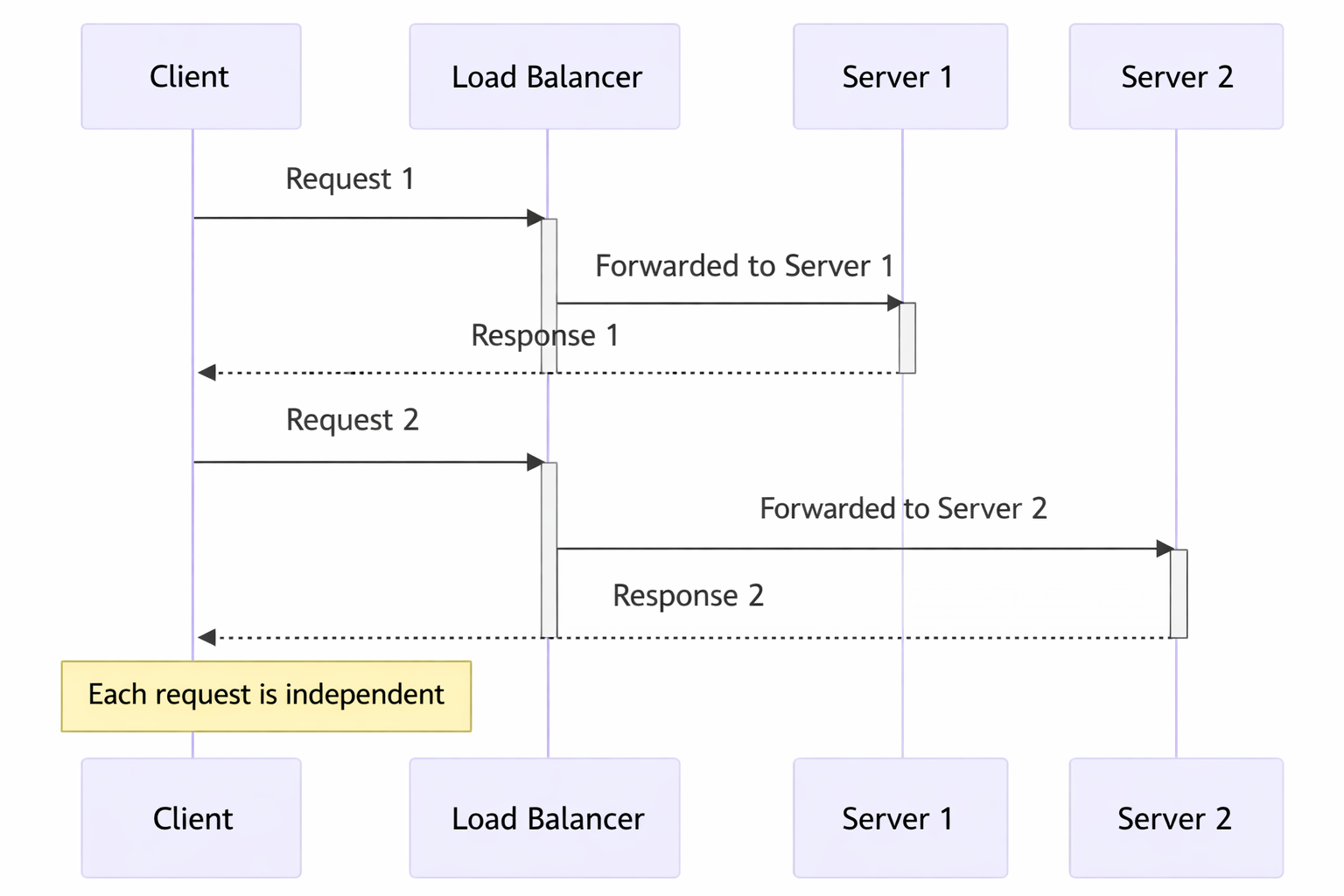
In this diagram:
Request 1: The client sends a request to the load balancer.
Load Balancer to Server 1: The load balancer forwards Request 1 to Server 1.
Response from Server 1: Server 1 processes the request and sends a response back to the client.
Request 2: The client sends another request to the load balancer.
Load Balancer to Server 2: This time, the load balancer forwards Request 2 to Server 2.
Response from Server 2: Server 2 processes the request and responds to the client.
Statelessness: Each request is independent and does not rely on previous interactions. Different servers can handle other requests without needing a shared session state.
Token-Based Authentication
Common in stateless architectures, this method involves passing a token for authentication with each request instead of relying on server-stored session data. JWT (JSON Web Tokens) is a popular example.
[Avg. reading time: 2 minutes]
Idempotency
In simple terms, idempotency is the property where an operation can be applied multiple times without changing the result beyond the initial application.
Think of an elevator button: whether you press it once or mash it ten times, the elevator is still only called once to your floor. The first press changed the state; the subsequent ones are “no-ops.”
In technology, this is the “secret sauce” for reliability. If a network glitch occurs and a request is retried, idempotency ensures you don’t end up with duplicate orders, double payments, or corrupted data.
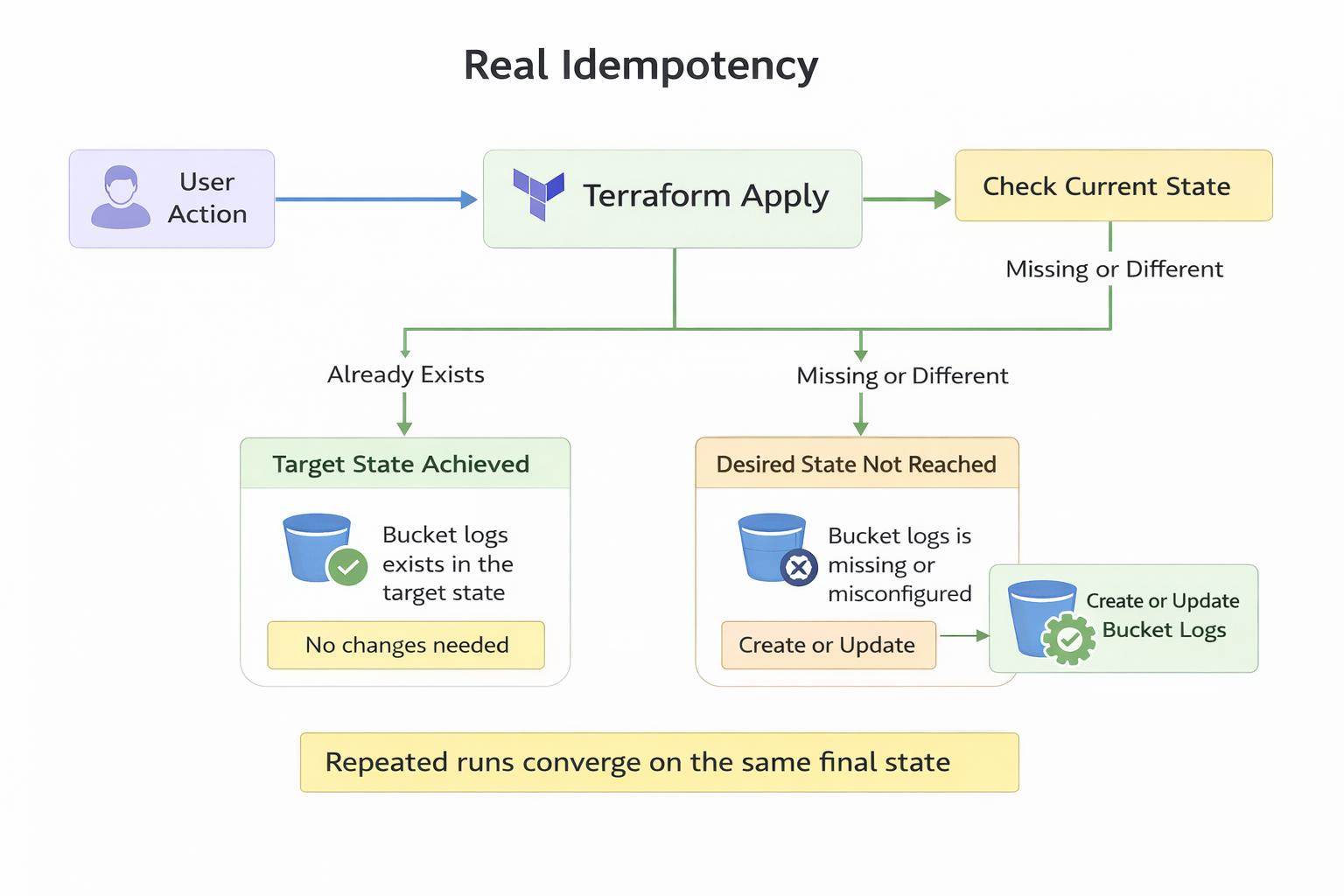
Popular Examples
- The MERGE (Upsert) Operation
- ABS(-5)
- Using Terraform to deploy server
#idempotent #merge #upsert #teraform #abs
[Avg. reading time: 8 minutes]
REST API
REpresentational State Transfer is a software architectural style developers apply to web APIs.
REST APIs provide simple, uniform interfaces because they can be used to make data, content, algorithms, media, and other digital resources available through web URLs. Essentially, REST APIs are the most common APIs used across the web today.
Use of a uniform interface (UI)
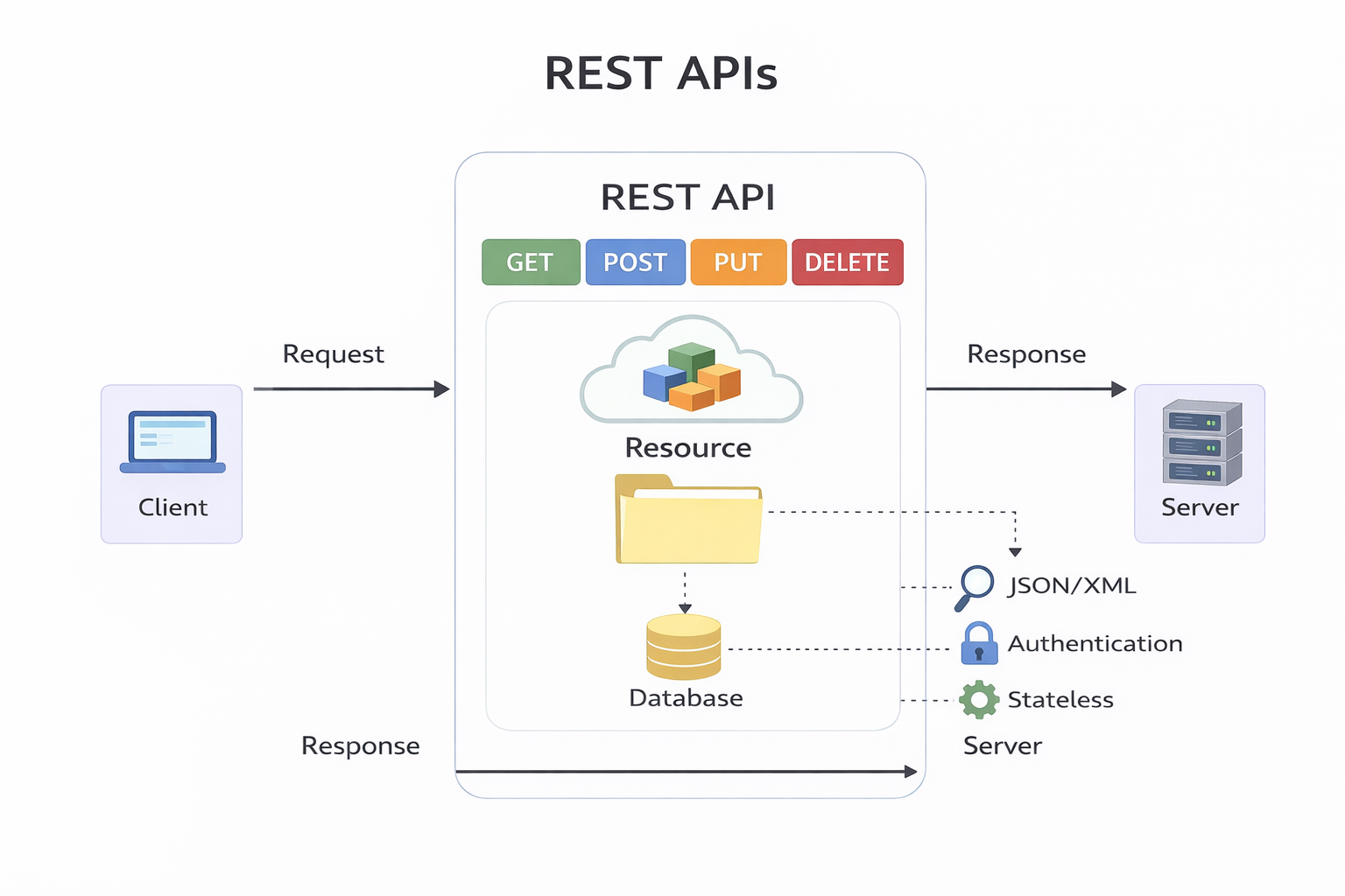
HTTP Methods
GET: This method allows the server to find the data you requested and send it back to you.
POST: This method permits the server to create a new entry in the database.
PUT: If you perform the ‘PUT’ request, the server will update an entry in the database.
DELETE: This method allows the server to delete an entry in the database.
Sample REST API URI
https://api.zippopotam.us/us/08028

http://api.tvmaze.com/search/shows?q=friends

https://jsonplaceholder.typicode.com/posts

https://jsonplaceholder.typicode.com/posts/1

https://jsonplaceholder.typicode.com/posts/1/comments

https://reqres.in/api/users?page=2

https://reqres.in/api/users/2

http://universities.hipolabs.com/search?country=United+States

https://itunes.apple.com/search?term=michael&limit=1000

https://www.boredapi.com/api/activity

https://techcrunch.com/wp-json/wp/v2/posts?per_page=100&context=embed
Usage
curl https://api.zippopotam.us/us/08028
curl https://api.zippopotam.us/us/08028 -o zipdata.json
Browser based
VS Code based
Python way
using requests library
Summary
Definition: REST (Representational State Transfer) API is a set of guidelines for building web services. A RESTful API is an API that adheres to these guidelines and allows for interaction with RESTful web services.
How It Works: REST uses standard HTTP methods like GET, POST, PUT, DELETE, etc. It is stateless, meaning each request from a client to a server must contain all the information needed to understand and complete the request.
Data Format: REST APIs typically exchange data in JSON or XML format.
Purpose: REST APIs are designed to be a simple and standardized way for systems to communicate over the web. They enable the backend services to communicate with front-end applications (like SPAs) or other services.
Use Cases: REST APIs are used in web services, mobile applications, and IoT (Internet of Things) applications for various purposes like fetching data, sending commands, and more.
#restapi #REST #curl #requests
[Avg. reading time: 6 minutes]
API Performance
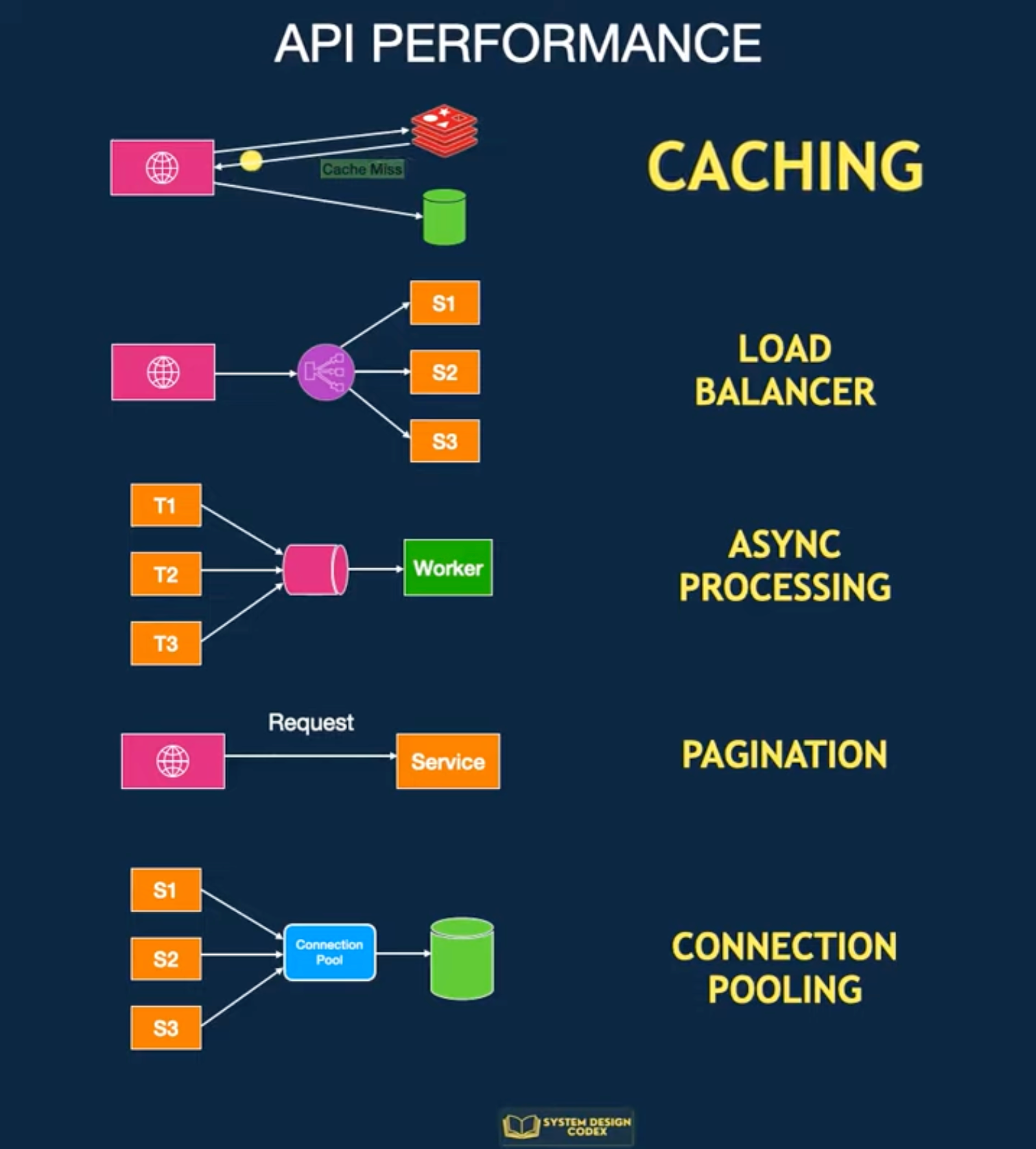
Caching
Store frequently accessed data in a cache so you can access it faster.
If there’s a cache miss, fetch the data from the database.
It’s pretty effective, but it can be challenging to invalidate and decide on the caching strategy.
Scale-out with Load Balancing
You can consider scaling your API to multiple servers if one server instance isn’t enough. Horizontal scaling is the way to achieve this.
The challenge will be to find a way to distribute requests between these multiple instances.
Load Balancing
It not only helps with performance but also makes your application more reliable.
However, load balancers work best when your application is stateless and easy to scale horizontally.
Pagination
If your API returns many records, you need to explore Pagination.
You limit the number of records per request.
This improves the response time of your API for the consumer.
Async Processing
With async processing, you can let the clients know that their requests are registered and under process.
Then, you process the requests individually and communicate the results to the client later.
This allows your application server to take a breather and give its best performance.
But of course, async processing may not be possible for every requirement.
Connection Pooling
An API often needs to connect to the database to fetch some data.
Creating a new connection for each request can degrade performance.
It’s a good idea to use connection pooling to set up a pool of database connections that can be reused across requests.
This is a subtle aspect, but connection pooling can dramatically impact performance in highly concurrent systems.
#api #performance #loadbalancing #pagination #connectionpool
[Avg. reading time: 4 minutes]
API in Big Data World
Big data and REST APIs are often used together in modern data architectures. Here’s how they interact:
Ingestion gateway
- Applications push events through REST endpoints
- Gateway converts to Kafka, Kinesis, or file landing zones
- REST is entry door, not the pipeline itself
Serving layer
- Processed data in Hive, Elasticsearch, Druid, or Delta
- APIs expose aggregated results to apps and dashboards
- REST is read interface on top of heavy compute
Control plane
- Spark job submission via REST
- Kafka topic management
- cluster monitoring and scaling
- authentication and governance
Microservices boundary
- Each service owns a slice of data
- APIs expose curated views
- internal pipelines stay streaming or batch
What REST is NOT in Big Data
- Not used for bulk petabyte transfer
- Not used inside Spark transformations
- Not the transport between Kafka and processors
Example of API in Big Data
https://docs.redis.com/latest/rs/references/rest-api/
https://rapidapi.com/search/big-data
https://www.kaggle.com/discussions/general/315241
[Avg. reading time: 2 minutes]
Advance Python
[Avg. reading time: 21 minutes]
Data Frames
DataFrames are the core abstraction for tabular data in analytics, machine learning, and ETL systems.
Think of a DataFrame as:
- A database table
- An Excel sheet
- A SQL result set
- A structured dataset in memory
But with a programmable API.
Using Data Frames helps you to
- Select columns
- Filter rows
- Aggregate data
- Join datasets
- Transform data efficiently
- Read and write formats like CSV, Parquet, JSON, Arrow
A DataFrame is:
- Column-oriented
- Vectorized
- Designed for batch transformations
- Not meant for row-by-row Python loops
Wrong Idea
for row in df:
    total = price * quantity
Correct Idea
You think in transformations, no iteration.
df["total"] = df["price"] * df["quantity"]
Pandas
Pandas is a popular Python library for data manipulation and analysis. A DataFrame in Pandas is a two-dimensional, size-mutable, and heterogeneous tabular data structure with labeled axes (rows and columns).
Eager Evaluation: Pandas performs operations eagerly, meaning that each operation is executed immediately when called.
In-Memory Copy - Full DataFrame in RAM, single copy
Sequential Processing - Single threaded, one operation at at time.
Strengths
- Extremely intuitive API
- Huge ecosystem
- Excellent for exploration
- Strong integration with ML libraries
- Perfect for small to medium datasets
Weaknesses
- Limited by RAM
- Single-core execution
- Slow for very large datasets
- No query optimizer
Example
import pandas as pd

df = pd.read_csv("data/sales_100.csv")

# Filter
filtered = df[df["region"] == "East"]

# Group and aggregate
result = filtered.groupby("category")["sales"].sum()

print(result.head())
When not to use Pandas
- Data exceeds available memory
- Computations become slow
- CPU only uses one core
- Processing large CSV files takes too long
Polars
Polars is a fast, multi-threaded DataFrame library in Rust and Python, designed for performance and scalability. It is known for its efficient handling of larger-than-memory datasets.
Supports both eager and lazy evaluation.
Lazy Evaluation: Instead of loading the entire CSV file into memory right away, a Lazy DataFrame builds a blueprint or execution plan describing how the data should be read and processed. The actual data is loaded only when the computation is triggered (for example, when you call a collect or execute command).
Optimizations: Using scan_csv allows Polars to optimize the entire query pipeline before loading any data. This approach is beneficial for large datasets because it minimizes memory usage and improves execution efficiency.
- pl.read_csv() or pl.read_parquet() - eager evaluation
- pl.scan_csv() or pl.scan_parquet() - lazy evaluation
Parallel Execution: Multi-threaded compute.
Columnar efficiency: Uses Arrow columnar memory format under the hood.
Pros
- High performance due to multi-threading and memory-efficient execution.
- Lazy evaluation, optimizing the execution of queries.
- Handles larger datasets effectively.
Cons
- Smaller community and ecosystem compared to Pandas.
- Less mature with fewer third-party integrations.
Example
import polars as pl

# Load the CSV file using Polars
df = pl.scan_csv('data/sales_100.csv')

print(df.head())

# Display the first few rows
print(df.collect())

df1 = pl.read_csv('data/sales_100.csv')
print(df1.head())
Dask
Dask is a parallel computing library that scales Python libraries like Pandas for large, distributed datasets.
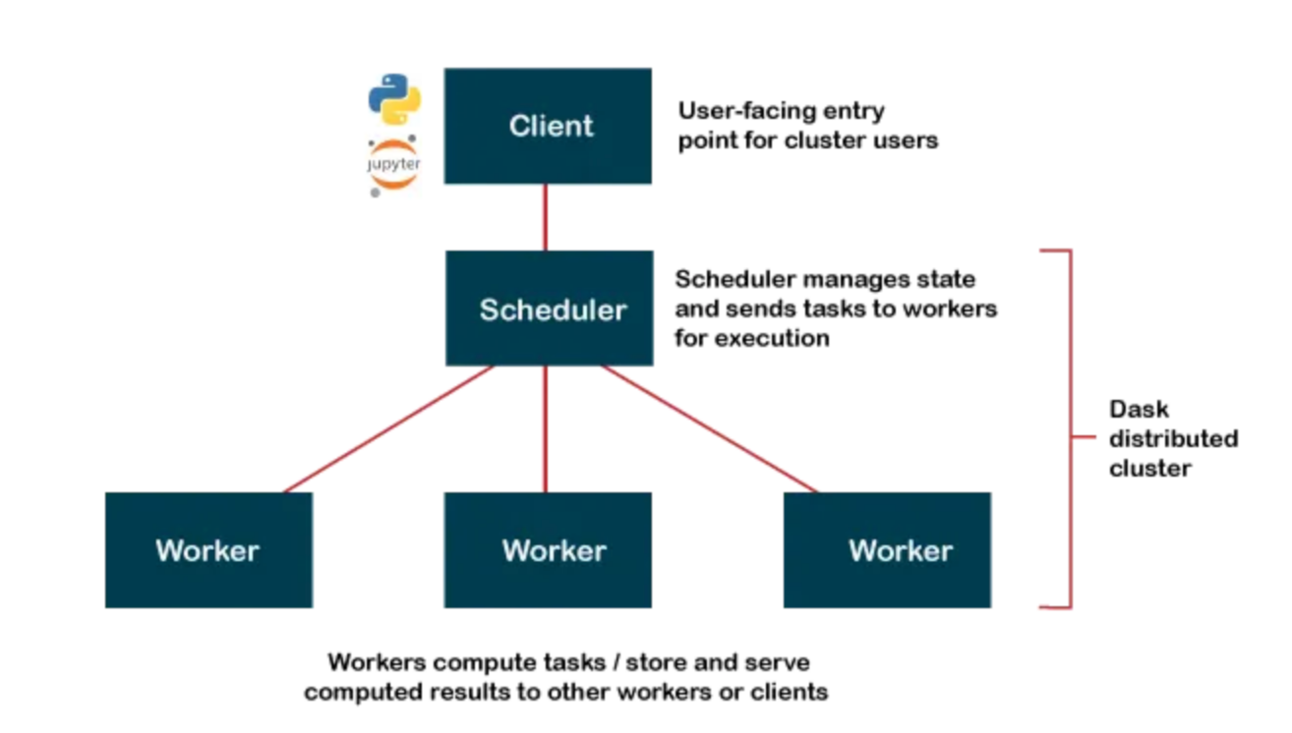
Client (Python Code)
   │
   ▼
Scheduler (builds + manages task graph)
   │
   ▼
Workers (execute tasks in parallel)
   │
   ▼
Results gathered back to client
Open Source https://docs.dask.org/en/stable/install.html
Dask Cloud Coiled Cloud
Lazy Reading: Dask builds a task graph instead of executing immediately — computations run only when triggered (similar to Polars lazy execution).
Partitioning: A Dask DataFrame is split into many smaller Pandas DataFrames (partitions) that can be processed in parallel.
Task Graph: Dask represents your workflow as a directed acyclic graph (DAG) showing the sequence and dependencies of tasks.
Distributed Compute: Dask executes tasks across multiple cores or machines, enabling scalable, parallel data processing.
import dask.dataframe as dd

ddf = dd.read_csv(
    "data/sales_*.csv",
    dtype={"category": "string", "value": "float64"},
    blocksize="64MB"
)

# 2) Lazy transform: per-partition groupby + sum, then global combine
agg = ddf.groupby("category")["value"].sum().sort_values(ascending=False)

# 3) Trigger execution and bring small result to driver
result = agg.compute()

print(result.head(10))
blocksize determines the parition. If omitted dask automatically uses 64MB
flowchart LR
  A1[CSV part 1] --> P1[parse p1]
  A2[CSV part 2] --> P2[parse p2]
  A3[CSV part 3] --> P3[parse p3]

  P1 --> G1[local groupby-sum p1]
  P2 --> G2[local groupby-sum p2]
  P3 --> G3[local groupby-sum p3]

  G1 --> C[combine-aggregate]
  G2 --> C
  G3 --> C

  C --> S[sort values]
  S --> R[collect to Pandas]
Pros
- Can handle datasets that don’t fit into memory by processing in parallel.
- Scales to multiple cores and clusters, making it suitable for big data tasks.
- Integrates well with Pandas and other Python libraries.
Cons
- Slightly more complex API compared to Pandas.
- Performance tuning can be more challenging.
Where to start?
- Start with Pandas for learning and small datasets.
- Switch to Polars when performance matters.
- Use Dask when data exceeds single-machine memory or needs cluster execution.
Pandas vs Polars vs Dask
| Feature | Pandas | Polars | Dask |
|---|---|---|---|
| Language | Python | Rust with Python bindings | Python |
| Execution Model | Single-threaded | Multi-threaded | Multi-threaded, distributed |
| Data Handling | In-memory | In-memory, Arrow-based | In-memory, out-of-core |
| Scalability | Limited by memory | Limited to single machine | Scales across clusters |
| Performance | Good for small to medium data | High performance for single machine | Good for large datasets |
| API Familiarity | Widely known, mature | Similar to Pandas | Similar to Pandas |
| Ease of Use | Very easy, large ecosystem | Easy, but smaller ecosystem | Moderate, requires understanding of parallelism |
| Fault Tolerance | None | Limited | High, with task retries and rescheduling |
| Machine Learning | Integration with Python ML libs | Preprocessing only | Integration with Dask-ML and other libs |
| Lazy Evaluation | No | Yes | Yes, with task graphs |
| Best For | Data analysis, small datasets | Fast preprocessing on single machine | Large-scale data processing |
| Cluster Management | N/A | N/A | Supports Kubernetes, YARN, etc. |
| Use Cases | Data manipulation, analysis | Fast data manipulation | Large data, ETL, scaling Python code |
[Avg. reading time: 16 minutes]
Decorator
Decorators in Python are a powerful way to modify or extend the behavior of functions or methods without changing their code. Decorators are often used for tasks like logging, authentication, and adding additional functionality to functions. They are denoted by the “@” symbol and are applied above the function they decorate.
def say_hello():
    print("World")

say_hello()
How do we change the output without changing the say hello() function?
wrapper() is not reserved word. It can be anyting.
Use Decorators
# Define a decorator function
def hello_decorator(func):
    def wrapper():
        print("Hello,")
        func()  # Call the original function
    return wrapper

# Use the decorator to modify the behavior of say_hello
@hello_decorator
def say_hello():
    print("World")

# Call the decorated function
say_hello()
If you want to replace the new line character and the end of the print statement, use end=''
# Define a decorator function
def hello_decorator(func):
    def wrapper():
        print("Hello, ", end='')
        func()  # Call the original function
    return wrapper

# Use the decorator to modify the behavior of say_hello
@hello_decorator
def say_hello():
    print("World")

# Call the decorated function
say_hello()
Multiple functions inside the Decorator
def hello_decorator(func):
    def first_wrapper():
        print("First wrapper, doing something before the second wrapper.")
        #func()

    def second_wrapper():
        print("Second wrapper, doing something before the actual function.")
        #func()

    def main_wrapper():
        first_wrapper()  # Call the first wrapper
        second_wrapper()  # Then call the second wrapper, which calls the actual function
        func()

    return main_wrapper

@hello_decorator
def say_hello():
    print("World")

say_hello()
Args & Kwargs
*args: This is used to represent positional arguments. It collects all the positional arguments passed to the decorated function as a tuple.**kwargs: This is used to represent keyword arguments. It collects all the keyword arguments (arguments passed with names) as a dictionary.
from functools import wraps

def my_decorator(func):
    @wraps(func)
    def wrapper(*args, **kwargs):
        print("Positional Arguments (*args):", args)
        print("Keyword Arguments (**kwargs):", kwargs)
        result = func(*args, **kwargs)
        return result
    return wrapper

@my_decorator
def example_function(a, b, c=0, d=0):
    print("Function Body:", a, b, c, d)

# Calling the decorated function with different arguments
example_function(1, 2)
example_function(3, 4, c=5)
Popular Example
Without Wraps
import time
import random
from functools import wraps

def timer(func):
    def wrapper(*args, **kwargs):
        name = wrapper.__name__
        start = time.perf_counter()
        result = func(*args, **kwargs)
        end = time.perf_counter()
        print(f"{name} took {end - start:.6f} seconds")
        return result
    return wrapper


@timer
def built_in_sort(data):
    return sorted(data)


@timer
def bubble_sort(data):
    arr = data.copy()
    n = len(arr)
    for i in range(n):
        for j in range(0, n - i - 1):
            if arr[j] > arr[j + 1]:
                arr[j], arr[j + 1] = arr[j + 1], arr[j]
    return arr


data = [random.randint(1, 100000) for _ in range(5000)]

built_in_sort(data)
bubble_sort(data)
Using Wraps
import time
import random
from functools import wraps

def timer(label=None):
    def decorator(func):
        @wraps(func)
        def wrapper(*args, **kwargs):
            name = label or wrapper.__name__
            start = time.perf_counter()
            result = func(*args, **kwargs)
            end = time.perf_counter()
            print(f"{name} took {end - start:.6f} seconds")
            return result
        return wrapper
    return decorator


@timer()
def built_in_sort(data):
    return sorted(data)


@timer("Custom Bubble Sort")
def bubble_sort(data):
    arr = data.copy()
    n = len(arr)
    for i in range(n):
        for j in range(0, n - i - 1):
            if arr[j] > arr[j + 1]:
                arr[j], arr[j + 1] = arr[j + 1], arr[j]
    return arr


data = [random.randint(1, 100000) for _ in range(5000)]

built_in_sort(data)
bubble_sort(data)
The purpose of @wraps is to preserve the metadata of the original function being decorated.
[Avg. reading time: 3 minutes]
Unit Testing
A unit test tests a small “unit” of code - usually a function or method - independently from the rest of the program.
Some key advantages of unit testing include:
- Isolates code - This allows testing individual units in isolation from other parts of the codebase, making bugs easier to identify.
- Early detection - Tests can catch issues early in development before code is deployed, saving time and money.
- Regression prevention - Existing unit tests can be run whenever code is changed to prevent new bugs or regressions.
- Facilitates changes - Unit tests give developers the confidence to refactor or update code without breaking functionality.
- Quality assurance - High unit test coverage helps enforce quality standards and identify edge cases.
Every language has its unit testing framework. In Python, some popular ones are
- unittest
- pytest
- doctest
- testify
Example:
Using Pytest & UV
git clone https://github.com/gchandra10/pytest-demo.git
[Avg. reading time: 8 minutes]
Error Handling
Python uses try/except blocks for error handling.
The basic structure is:
try:
    # Code that may raise an exception
except ExceptionType:
    # Code to handle the exception
finally:
    # Code executes all the time
Uses
Improved User Experience: Instead of the program crashing, you can provide a user-friendly error message.
Debugging: Capturing exceptions can help you log errors and understand what went wrong.
Program Continuity: Allows the program to continue running or perform cleanup operations before terminating.
Guaranteed Cleanup: Ensures that certain operations, like closing files or releasing resources, are always performed.
Some key points
-
You can catch specific exception types or use a bare except to catch any exception.
-
Multiple except blocks can be used to handle different exceptions.
-
An else clause can be added to run if no exception occurs.
-
A finally clause will always execute, whether an exception occurred or not.
Without Try/Except
x = 10 / 0
Basic Try/Except
try:
    x = 10 / 0
except ZeroDivisionError:
    print("Error: Division by zero!")
Generic Exception
try:
    file = open("nonexistent_file.txt", "r")
except:
    print("An error occurred!")
Find the exact error
try:
    file = open("nonexistent_file.txt", "r")
except Exception as e:
    print(str(e))
Raise - Else and Finally
try:
    x = -10
    if x <= 0:
        raise ValueError("Number must be positive")
except ValueError as ve:
    print(f"Error: {ve}")
else:
    print(f"You entered: {x}")
finally:
    print("This will always execute")
try:
    x = 10
    if x <= 0:
        raise ValueError("Number must be positive")
except ValueError as ve:
    print(f"Error: {ve}")
else:
    print(f"You entered: {x}")
finally:
    print("This will always execute")
Nested Functions
def divide(a, b):
    try:
        result = a / b
        return result
    except ZeroDivisionError:
        print("Error in divide(): Cannot divide by zero!")
        raise  # Re-raise the exception

def calculate_and_print(x, y):
    try:
        result = divide(x, y)
        print(f"The result of {x} divided by {y} is: {result}")
    except ZeroDivisionError as e:
        print(str(e))
    except TypeError as e:
        print(str(e))

# Test the nested error handling
print("Example 1: Valid division")
calculate_and_print(10, 2)

print("\nExample 2: Division by zero")
calculate_and_print(10, 0)

print("\nExample 3: Invalid type")
calculate_and_print("10", 2)
#errorhandling #exception #try
[Avg. reading time: 7 minutes]
Logging
Python’s logging module provides a flexible framework for tracking events in your applications. It’s used to log messages to various outputs (console, files, etc.) with different severity levels like DEBUG, INFO, WARNING, ERROR, and CRITICAL.
Use Cases of Logging
Debugging: Identify issues during development. Monitoring: Track events in production to monitor behavior. Audit Trails: Capture what has been executed for security or compliance. Error Tracking: Store errors for post-mortem analysis. Rotating Log Files: Prevent logs from growing indefinitely using size or time-based rotation.
Python Logging Levels
| Level | Usage | Numeric Value | Description |
|---|---|---|---|
DEBUG | Detailed information for diagnosing problems. | 10 | Useful during development and debugging stages. |
INFO | General information about program execution. | 20 | Highlights normal, expected behavior (e.g., program start, process completion). |
WARNING | Indicates something unexpected but not critical. | 30 | Warns of potential problems or events to monitor (e.g., deprecated functions, nearing limits). |
ERROR | An error occurred that prevented some part of the program from working. | 40 | Represents recoverable errors that might still allow the program to continue running. |
CRITICAL | Severe errors indicating a major failure. | 50 | Marks critical issues requiring immediate attention (e.g., system crash, data corruption). |
INFO
import logging

logging.basicConfig(level=logging.INFO)  # Set the logging level to INFO

logging.debug("This is a debug message.")
logging.info("This is an info message.")
logging.warning("This is a warning message.")
logging.error("This is an error message.")
logging.critical("This is a critical message.")
Error
import logging

logging.basicConfig(level=logging.ERROR)  # Set the logging level to ERROR

logging.debug("This is a debug message.")
logging.info("This is an info message.")
logging.warning("This is a warning message.")
logging.error("This is an error message.")
logging.critical("This is a critical message.")
import logging

logging.basicConfig(
    level=logging.DEBUG,
    format = '%(asctime)s - %(name)s - %(levelname)s - %(message)s'
)

logging.debug("This is a debug message.")
logging.info("This is an info message.")
logging.warning("This is a warning message.")
More Examples
git clone https://github.com/gchandra10/python_logging_examples.git
[Avg. reading time: 0 minutes]
Containers
- CPU Architecture Fundamentals
- Introduction
- VMs or Containers
- What Container does
- Docker
- Docker Examples
[Avg. reading time: 8 minutes]
CPU Architecture Fundamentals
Introduction
CPU architecture defines:
- The instruction set a processor understands
- Register structure
- Memory addressing model
- Binary format
It determines what machine code can run on a processor.
If software is compiled for one architecture, it cannot run on another without translation.
Major CPU Architectures
In todays world.
1. amd64 (x86_64)
- Designed by AMD, adopted by Intel
- Dominates desktops and traditional servers
- Common in enterprise data centers
- Most Windows laptops
- Intel-based Macs
Characteristics:
- High performance
- Higher power consumption
2. arm64 (aarch64)
- Designed for power efficiency
- Common in embedded systems and mobile devices
- Raspberry Pi
- Apple Silicon (M*)
- Many IoT gateways
Characteristics:
- Energy efficient
- Dominant in IoT and edge computing
Mac/Linux
uname -m
Windows
echo %%PROCESSOR_ARCHITECTURE%%
systeminfo | findstr /B /C:"System Type"
How Programming Languages Relate to Architecture
                +----------------------+
                |     Source Code      |
                |  (C, Rust, Python)   |
                +----------+-----------+
                           |
                           v
                +----------------------+
                |     Compiler /       |
                |     Interpreter      |
                +----------+-----------+
                           |
         +-----------------+-----------------+
         |                                   |
         v                                   v
+---------------------+          +----------------------+
|  amd64 Binary       |          |  arm64 Binary       |
|  (x86_64 machine    |          |  (ARM machine       |
|   instructions)     |          |   instructions)     |
+----------+----------+          +----------+-----------+
           |                                |
           v                                v
+---------------------+          +----------------------+
|  Intel / AMD CPU    |          |  ARM CPU            |
|  (Laptop, Server)   |          |  (Raspberry Pi,     |
|                     |          |   IoT Gateway)      |
+---------------------+          +----------------------+
Compiled Languages
Examples: C, C++, Rust, Go
When compiled, they produce native machine code.
Compile on Windows - produces an amd64 binary.
Compile on Raspberry Pi or new Mac - produces an arm64 binary.
That binary cannot run on a different architecture.
Interpreted Languages
Examples: Python, Node.js
Source code is architecture-neutral. Interpreter handles it.
The interpreter (Python, Node) is architecture-specific
Native extensions are architecture-specific.
Java and Bytecode
            +------------------+
            |   Java Source    |
            +--------+---------+
                     |
                     v
            +------------------+
            |    Bytecode      |
            |   (.class file)  |
            +--------+---------+
                     |
         +-----------+-----------+
         |                       |
         v                       v
+------------------+     +------------------+
| JVM (amd64)      |     | JVM (arm64)      |
+--------+---------+     +--------+---------+
         |                        |
         v                        v
   Intel CPU                ARM CPU
Java uses a different model.
Compile: javac MyApp.java
Produces: MyApp.class
This is bytecode, not native machine code.
Bytecode runs on the JVM (Java Virtual Machine).
The JVM is architecture-specific.
Same bytecode runs on amd64 JVM
Same bytecode runs on arm64 JVM
Java achieves portability through a virtual machine layer.
Cross Compilation
It is possible to cross compile for a different architecture than your current architecture.
Developer Laptop (amd64)
        |
        | build
        v
   amd64 binary
        |
        | deploy
        v
Raspberry Pi (arm64)
        |
        X  Fails (architecture mismatch)
Developer Laptop
        |
        | cross-build for arm64
        v
   arm64 binary
        |
        v
Raspberry Pi (runs successfully)
Architecture in IoT Upper Stack
| Layer | Typical Architecture |
|---|---|
| Microcontroller | ARM (32-bit or 64-bit) |
| Edge Gateway | arm64 |
| Cloud VM | amd64 or arm64 |
| Personal Machines | amd64 or arm64 |
[Avg. reading time: 6 minutes]
Containers
World before containers
Physical Machines
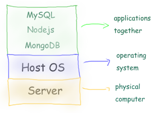
- 1 Physical Server
- 1 Host Machine (say some Linux)
- 3 Applications installed
Limitation:
- Need of physical server.
- Version dependency (Host and related apps)
- Patches ”hopefully” not affecting applications.
- All apps should work with the same Host OS.
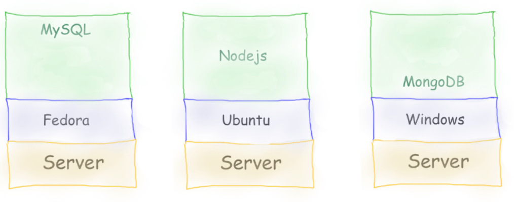
- 3 physical server
- 3 Host Machine (diff OS)
- 3 Applications installed
Limitation:
- Need of physical server(s).
- Version dependency (Host and related apps)
- Patches ”hopefully” not affecting applications.
- Maintenance of 3 machines.
- Network all three so they work together.
Virtual Machines
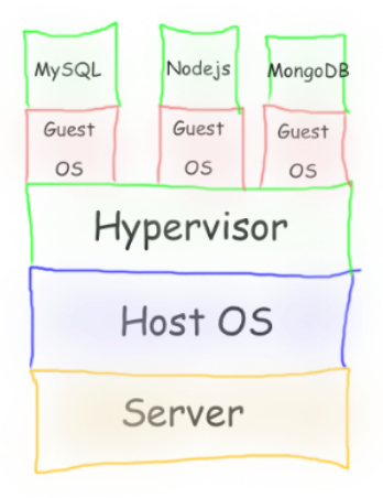
-
Virtual Machines emulate a real computer by virtualizing it to execute applications,running on top of a real computer.
-
To emulate a real computer, virtual machines use a Hypervisor to create a virtual computer.
-
On top of the Hypervisor, we have a Guest OS that is a Virtualized Operating System where we can run isolated applications, called Guest Operating System.
-
Applications that run in Virtual Machines have access to Binaries and Libraries on top of the operating system.
( + ) Full Isolation, Full virtualization
( - ) Too many layers, Heavy-duty servers.
Containers
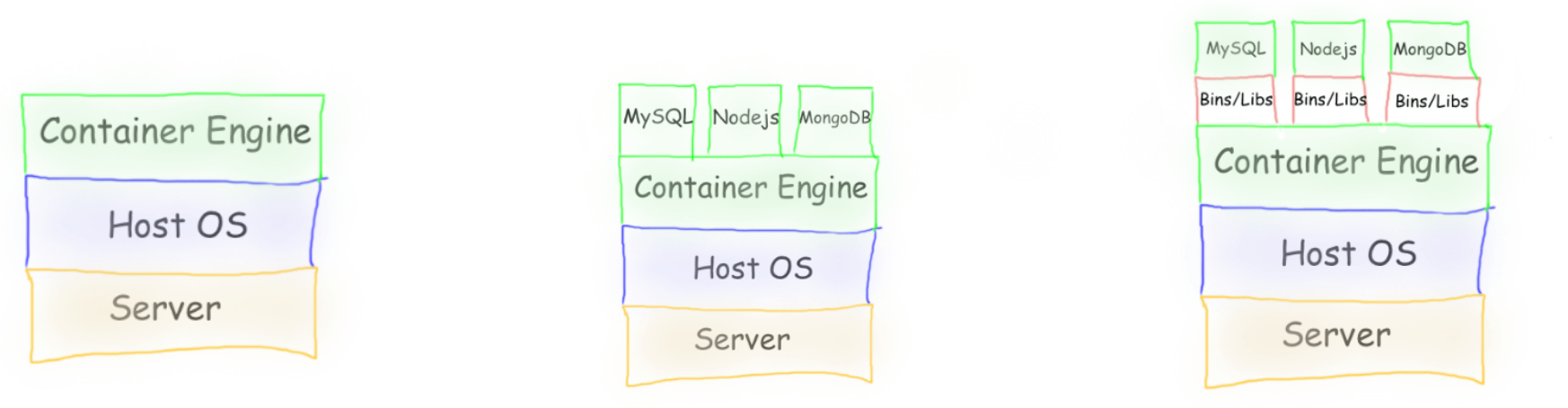
Containers are lightweight, portable environments that package an application with everything it needs to run—like code, runtime, libraries, and system tools—ensuring consistency across different environments. They run on the same operating system kernel and isolate applications from each other, which improves security and makes deployments easier.
-
Containers are isolated processes that share resources with their host and, unlike VMs, don’t virtualize the hardware and don’t need a Guest OS.
-
Containers share resources with other Containers in the same host.
-
This gives more performance than VMs (no separate guest OS).
-
Container Engine in place of Hypervisor.
Pros
- Isolated Process
- Mounted Files
- Lightweight Process
Cons
- Same Host OS
- Security
[Avg. reading time: 3 minutes]
VMs or Containers
VMs are great for running multiple, isolated OS environments on a single hardware platform. They offer strong security isolation and are useful when applications need different OS versions or configurations.
Containers are lightweight and share the host OS kernel, making them faster to start and less resource-intensive. They’re perfect for microservices, CI/CD pipelines, and scalable applications.
Smart engineers focus on the right tool for the job rather than getting caught up in “better or worse” debates.
Use them in combination to make life better.
Popular container technologies
Docker: The most widely used container platform, known for its simplicity, portability, and extensive ecosystem.
Podman: A daemonless container engine that’s compatible with Docker but emphasizes security, running containers as non-root users.
We will be using Docker for this course.
[Avg. reading time: 1 minute]
What container does
It brings to us the ability to create applications without worrying about their environment.

- Docker turns “my machine” into the machine
- Docker is not a magic want.
- It only guarantees the environment is identical
- Correctness still depends on what you build and how you run it.
#worksforme #container #docker
[Avg. reading time: 6 minutes]
Docker Basics
At a conceptual level, Docker is built around two core abstractions:
- Images – what you build
- Containers – what you run
Everything else in Docker exists to build, store, distribute, and execute these two artifacts.
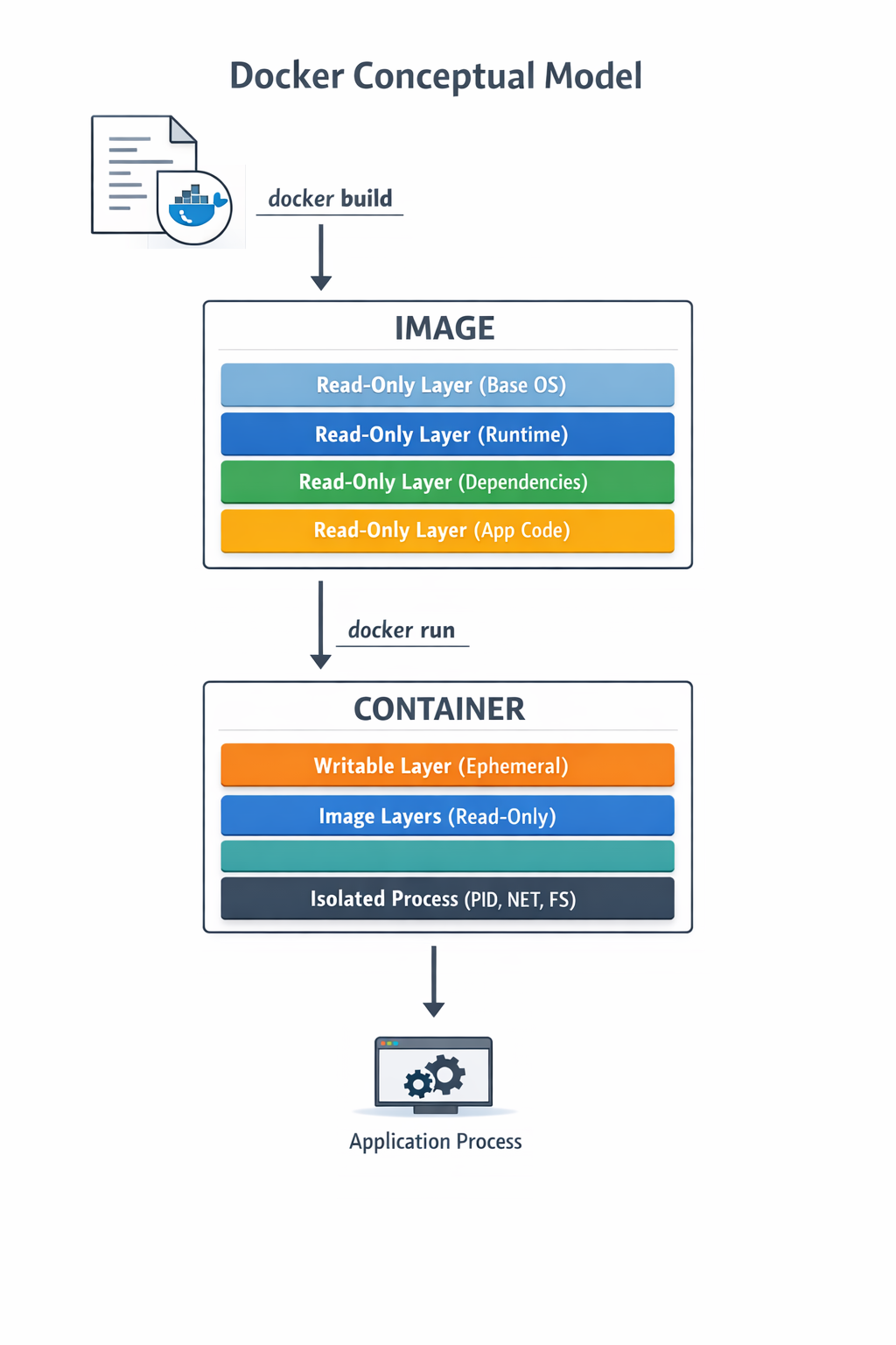
Images
- An image is an immutable, layered filesystem snapshot
- Built from a Dockerfile
- Each instruction creates a new read-only layer
- Images are content-addressed via SHA256 digests
Image is a versioned, layered blueprint
Key properties:
- Immutable
- Reusable
- Cached aggressively
- Portable across environments
Container
A container is a running instance of an image
- A writable layer on top of image layers
- Namespaces for isolation (PID, USER)
- Containers are processes, not virtual machines
- When the main process exits, the container stops
Image vs Container
| Aspect | Image | Container |
|---|---|---|
| Nature | Static | Dynamic |
| Mutability | Immutable | Mutable |
| Lifecycle | Build-time | Runtime |
| Role | Artifact | Instance |
Where Do Images Come From?
Docker Hub
- Default public container registry
- Hosts official and community images
- Supports tags, digests, vulnerability scans
- Docker Hub is default, not mandatory
Apart from Docker Hub, there are few other common registries
Private / On-Prem Registries
Enterprises widely use on-prem or private registries. JFrog Artifactory is extremely common in regulated environments.
#docker #container #repositories #hub
[Avg. reading time: 17 minutes]
Docker Examples
Mac Users
Open Terminal
Windows Users
Open Git Bash
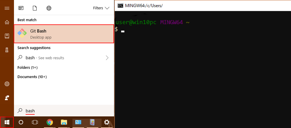
Is Docker Running?
docker info
- Lists images available on the local machine
docker image ls
- To get a specific image
docker image pull <imagename>
docker image pull python:3.12-slim
- To inspect the downloaded image
docker image inspect python:3.12-slim
Check the architecture, ports open etc..
- Create a container
docker create \
    --name edge-http \
    -p 8000:8000 \
    python:3.12-slim \
    python -m http.server
List the Image and container again
- Start the container
docker start edge-http
Open browser and check http://localhost:8000 shows the docker internal file structure.
docker inspect edge-http
- Shows all running containers
docker container ls
- Shows all containers
docker container ls -a
- Disk usage by images, containers, volumes
docker system df
- Logs Inspection
docker logs edge-http
docker inspect edge-http
- Stop and remove
docker stop edge-http
docker rm edge-http
docker run is a wrapper for docker pull, docker create, docker start
Deploy MySQL Database using Containers
Create the following folder
Linux / Mac
mkdir -p container/mysql
cd container/mysql
Windows
md container
cd container
md mysql
cd mysql
Note: If you already have MySQL Server installed in your machine then please change the port to 3307 as given below.
-p 3307:3306 \
Run the container
docker run --name mysql -d \
    -p 3306:3306 \
    -e MYSQL_ROOT_PASSWORD=root-pwd \
    -e MYSQL_ROOT_HOST="%" \
    -e MYSQL_DATABASE=mydb \
    -e MYSQL_USER=remote_user \
    -e MYSQL_PASSWORD=remote_user-pwd \
    docker.io/library/mysql:8.4.4
-d : detached (background mode) -p : 3306:3306 maps mysql default port 3306 to host machines port 3306 3307:3306 maps mysql default port 3306 to host machines port 3307
-e MYSQL_ROOT_HOST=“%” Allows to login to MySQL using MySQL Workbench
Login to MySQL Container
docker exec -it mysql bash
List all the Containers
docker container ls -a
Stop MySQL Container
docker stop mysql
Delete the container**
docker rm mysql
Preserve the Data for future
Inside container/mysql
mkdir data
docker run --name mysql -d \
    -p 3306:3306 \
    -e MYSQL_ROOT_PASSWORD=root-pwd \
    -e MYSQL_ROOT_HOST="%" \
    -e MYSQL_DATABASE=mydb \
    -e MYSQL_USER=remote_user \
    -e MYSQL_PASSWORD=remote_user-pwd \
    -v ./data:/var/lib/mysql \
    docker.io/library/mysql:8.4.4
-- Create database
CREATE DATABASE IF NOT EXISTS friends_tv_show;
USE friends_tv_show;

-- Create Characters table
CREATE TABLE characters (
    character_id INT AUTO_INCREMENT PRIMARY KEY,
    first_name VARCHAR(50) NOT NULL,
    last_name VARCHAR(50) NOT NULL,
    actor_name VARCHAR(100) NOT NULL,
    date_of_birth DATE,
    occupation VARCHAR(100),
    apartment_number VARCHAR(10)
);

INSERT INTO characters (first_name, last_name, actor_name, date_of_birth, occupation, apartment_number) VALUES
('Ross', 'Geller', 'David Schwimmer', '1967-10-02', 'Paleontologist', '3B'),
('Rachel', 'Green', 'Jennifer Aniston', '1969-02-11', 'Fashion Executive', '20'),
('Chandler', 'Bing', 'Matthew Perry', '1969-08-19', 'IT Procurement Manager', '19'),
('Monica', 'Geller', 'Courteney Cox', '1964-06-15', 'Chef', '20'),
('Joey', 'Tribbiani', 'Matt LeBlanc', '1967-07-25', 'Actor', '19'),
('Phoebe', 'Buffay', 'Lisa Kudrow', '1963-07-30', 'Massage Therapist/Musician', NULL);

select * from characters;
Build your own Image
mkdir -p container
cd container
Python Example
Follow the README.md
Fork & Clone
git clone https://github.com/gchandra10/docker_mycalc_demo.git
Web App Demo
Fork & Clone
git clone https://github.com/gchandra10/docker_webapp_demo.git
Docker Compose
Docker Compose is a tool that lets you define and run multi-container Docker applications using a single YAML file.
Instead of manually running multiple docker run commands, you describe:
- Services (containers)
- Networks
- Volumes
- Environment variables
- Dependencies between services
…all inside a docker-compose.yml file.
Sample docker-compose.yaml
version: "3.9"

services:
  app:
    build: .
    ports:
      - "5000:5000"
    depends_on:
      - db

  db:
    image: postgres:15
    environment:
      POSTGRES_PASSWORD: example
docker compose up -d
docker compose down
Usecases
- Reproducible environments
- Clean dev setups
- Ideal for microservices
- Great for IoT stacks like broker + processor + DB
Docker Compose Demo
https://github.com/gchandra10/docker-compose-mysql-python-demo
Publish Image to Docker Hub
Login to Docker Hub
- Create a Repository “my_faker_calc”
- Under Account Settings
- Personal Access Token
- Create a PAT token with Read/Write access for 1 day
Replace gchandra10 with yours.
docker login

enter userid
enter PAT token
Then build the Image with your userid
docker build -t gchandra10/my_faker_calc:1.0 .
docker image ls
Copy the ImageID of gchandra10/my_fake_calc:1.0
Tag the ImageID with necessary version and latest
docker image tag <image_id> gchandra10/my_faker_calc:latest
Push the Images to Docker Hub (version and latest)
docker push gchandra10/my_faker_calc:1.0
docker push gchandra10/my_faker_calc:latest
Image Security
Trivy
Open Source Scanner.
https://trivy.dev/latest/getting-started/installation/
trivy image python:3.12-slim

# Focus on high risk only

trivy image --severity HIGH,CRITICAL python:3.12-slim

# Show only fixes available
trivy image --ignore-unfixed false python:3.12-slim

trivy image gchandra10/my_faker_calc

trivy image gchandra10/my_faker_calc --severity CRITICAL,HIGH --format table

trivy image gchandra10/my_faker_calc --severity CRITICAL,HIGH  --output result.txt
Grype
Open Source Scanner
grype python:3.12-slim
Common Mitigation Rules
- Upgrade the base
- move to newer version of python if 3.12 has issues
- Minimize OS packages
- check our how many layers of packages are installed
- Pin versions on libraries
- requirements.txt make sure Library versions are pinned for easy detection
- Run as non-root
- Create local user instead of running as root
- Don’t share Secrets
- dont copy .env or any secrets in your script or application.
[Avg. reading time: 0 minutes]
CICD
[Avg. reading time: 4 minutes]
CICD Intro
A CI/CD pipeline is a development practice focused on one core goal:
Ship high-quality features to production faster and more reliably.
Without CI/CD, every step in the software lifecycle is manual: building code, running tests, and deploying changes. This slows teams down and introduces human error.
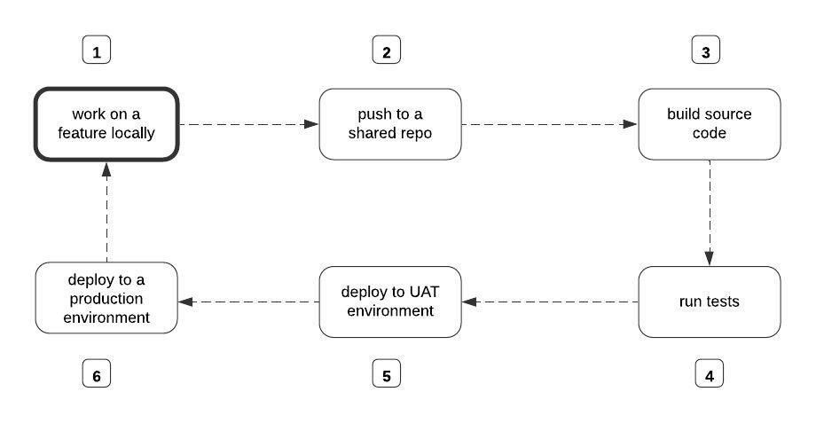 src: https://www.freecodecamp.org/
What Happens Without CI/CD?
- Developers manually trigger builds
- Testing is inconsistent or delayed
- Deployments are error-prone
- Releases take longer and break more often
CI/CD fixes this by automating the entire flow.
Continuous Integration (CI)
- Automatically builds and tests code whenever changes are pushed to a shared repository
- Detects issues early before they reach production
- Ensures new code doesn’t break existing functionality
Keep the codebase stable at all times
Continuous Delivery (CD)
- Automatically deploys validated code to staging or testing environments
- Production deployment is still a manual decision
Always be ready to release.
Continuous Deployment
- Extends Continuous Delivery
- Every successful change is automatically deployed to production
Remove manual steps and release continuously.
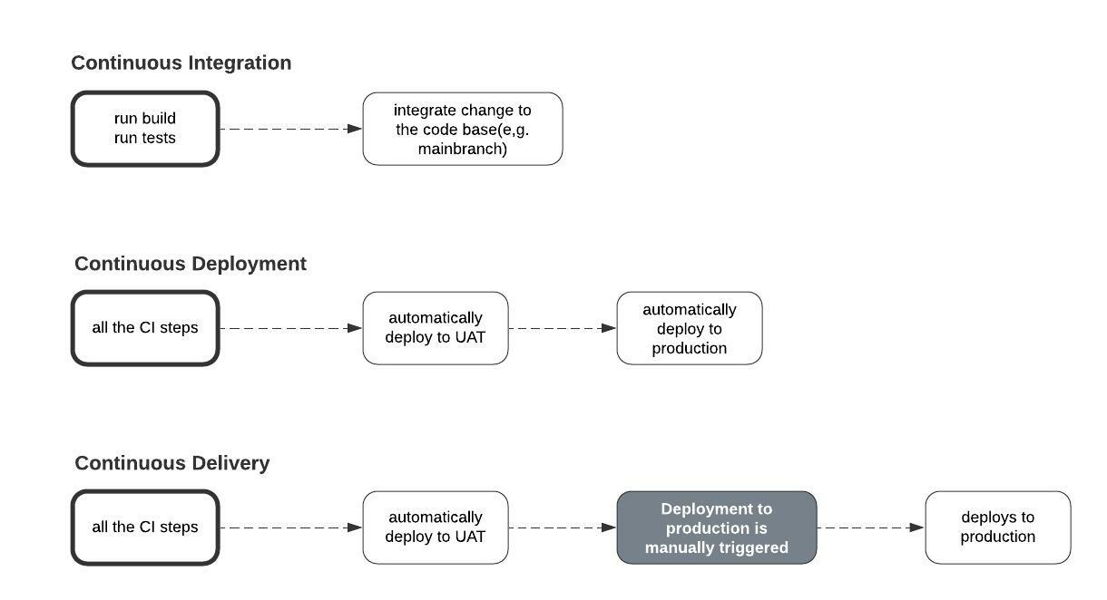
src 1
1: www.freecodecamp.org/
[Avg. reading time: 7 minutes]
CICD Tools
There are many CI/CD tools available. They differ mainly in hosting model and integration ecosystem.
Categories of CI/CD Tools
Self-Hosted / On-Prem
-
Jenkins
-
CircleCI (can be self-hosted, though mostly SaaS now)
-
You need full control
-
Strict security/compliance
-
Custom infrastructure
SaaS / Web-Based
-
GitHub Actions
-
GitLab CI/CD
-
You want quick setup
-
Tight integration with source control
Cloud-Native Tools
-
AWS CodeBuild / CodePipeline
-
Azure DevOps
-
Google Cloud Build
-
You’re already in that cloud
-
Need deep integration with cloud services
GitHub Actions
One of the most widely used CI/CD tools today.
- Native integration with GitHub
- Free tier available
- Huge marketplace of reusable actions
Core Five Concepts
Workflows
- Define the automation pipeline
- Stored as YAML files in .github/workflows/
- Think: entire pipeline definition
Jobs
- A workflow is made up of one or more jobs
- Jobs run independently (can be parallel)
- Each job contains multiple steps
Steps
- Individual tasks inside a job
- Example: install dependencies, run tests
Events (Triggers)
Trigger the execution of the job.
- on push / pull
- on schedule
- on workflow_dispatch (Manual Trigger)
Actions
Reusable building blocks.
Example:
- checkout repo
- setup Python
- deploy apps
https://github.com/features/actions
Runners
Remote computer that GitHub Actions uses to execute the jobs.
Github-Hosted Runners
- ubuntu-latest
- windows-latest
- macos-latest
Self-Hosted Runners
- Specific OS that Github does not offer.
- Connection to a private network/environment.
- To save costs for projects with high usage. (Enterprise plans are expensive)
YAML (Yet Another Markup Language)
- Human-readable
- Key-value structure
- Indentation matters
https://learnxinyminutes.com/docs/yaml/
Sample
name: CI Pipeline

on:
  push:
    branches: [main]
  pull_request:
    branches: [main]
  workflow_dispatch:
  schedule:
    - cron: '0 0 * * *'

jobs:
  build-and-test:
    runs-on: ubuntu-latest

    steps:
      - uses: actions/checkout@v4

      - name: Set up Python
        uses: actions/setup-python@v5
        with:
          python-version: '3.11'

      - name: Install dependencies
        run: |
          pip install -r requirements.txt

      - name: Run tests
        run: pytest
DEMO
Multiple Runners Demo
https://github.com/gchandra10/github-actions-multiple-runners-demo
https://github.com/gchandra10/python_cicd_calculator
[Avg. reading time: 4 minutes]
CI YAML
CI/CD is not just a tool or a YAML file. It is a system of interconnected components working together to ensure code quality.
checkout → install → test → notify
- CI is not about automation alone.
- It is about reducing the time between writing code and discovering problems.
- Faster feedback = better code quality
name: Build and Test

on:
  push:
    branches: [main]
  pull_request:
    branches: [main]
  workflow_dispatch:

permissions:
  contents: read

concurrency:
  group: ci-${{ github.ref }}
  cancel-in-progress: true

jobs:
  test:
    name: Test Calculator App
    runs-on: ubuntu-latest
    timeout-minutes: 10

    steps:
      - name: Checkout code
        uses: actions/checkout@v4

      - name: Set up Python environment
        uses: actions/setup-python@v6
        with:
          python-version: "3.11"
          cache: pip

      - name: Install dependencies
        run: |
          python -m pip install --upgrade pip
          pip install -r requirements.txt

      - name: Run tests
        run: |
          python -m unittest test_calc.py -v

      - name: Send Discord failure notification
        if: failure()
        env:
          DISCORD_WEBHOOK: ${{ secrets.DISCORD_WEBHOOK }}
        uses: Ilshidur/action-discord@0.4.0
        with:
          args: >
            @here The Calculator App integration test failed for
            ${{ github.repository }}.
            Check run ${{ github.run_id }} on GitHub for details.

      - name: Send Discord success notification
        if: success()
        env:
          DISCORD_WEBHOOK: ${{ secrets.DISCORD_WEBHOOK }}
        uses: Ilshidur/action-discord@0.4.0
        with:
          args: >
            The Calculator App for ${{ github.repository }}
            passed successfully.
            Run ID: ${{ github.run_id }}
[Avg. reading time: 2 minutes]
CD Yaml
    - name: Deploy to Server
      if: success()
      uses: appleboy/ssh-action@master
      with:
        host: ${{ secrets.SERVER_HOST }}
        username: ${{ secrets.SERVER_USER }}
        key: ${{ secrets.SSH_PRIVATE_KEY }}
        port: 22 # Optional if your SSH server uses a different port
        script: |
          cd /path/to/your/project
          git pull
          # Any other deployment or restart service commands
    - name: Configure AWS Credentials
      uses: aws-actions/configure-aws-credentials@v1
      with:
        aws-access-key-id: ${{ secrets.AWS_ACCESS_KEY_ID }}
        aws-secret-access-key: ${{ secrets.AWS_SECRET_ACCESS_KEY }}
        aws-region: your-aws-region

    - name: Deploy to AWS Lambda
      run: |
        # Package your application
        zip -r package.zip .
        # Deploy/update your Lambda function
        aws lambda update-function-code --function-name your-lambda-function-name --zip-file fileb://package.zip
[Avg. reading time: 1 minute]
Data Engineering
- Introduction
- Batch vs Streaming
- Medallion Architecture
- Data Quality Checks
- Data Engineering Model
- Quality & Governance
- Data Mesh
- KAFKA
[Avg. reading time: 2 minutes]
Introduction to Data Engineering
Data Engineering is not about dashboards or ML hype. It’s about building systems that move and shape data reliably at scale.
At its core, data engineering answers three questions:
- How does data enter the system
- How does it change as it moves
- How do we trust it when it’s used
Everything else is implementation detail.
Data comes from multiple sources:
- APIs
- Files (CSV, JSON, Parquet)
- Databases
- Streams
The real challenge is not loading data. It’s handling reality:
- Millions of records
- Partial failures
- Schema changes
- Late-arriving data
- Duplicate data
[Avg. reading time: 5 minutes]
Batch - Streaming - Microbatch
Batch Processing
Batch means collect first, process later.
- Works on large chunks of accumulated data
- High throughput, cheaper, simpler
- Results are not real-time
- Typically minutes, hours, or days delayed
Examples:
- Daily or weekly sales reports
- End-of-day stock portfolio reconciliation
- Monthly billing cycles
- ETL pipelines that refresh a data warehouse
Use cases
- Immediate action is not required
- Delay is acceptable
- Working with large historical datasets
Stream Processing
Streaming means process events the moment they arrive.
- Low-latency (milliseconds to seconds)
- Continuous, event-by-event processing
- Ideal for real-time analytics and alerting
- Stateful systems maintain event history or running context
Examples:
- Stock price updates
- Fraud detection for credit cards
- Real-time gaming leaderboards
- IoT sensor monitoring
Use cases
- You need instant reactions
- Delays cause risk, loss, or bad UX
Micro Batch
Micro-batching = small batches processed very frequently.
- Latency: ~0.5 to a few seconds
- Not true real-time, but close
- Simpler than full streaming
- Common in systems like Spark Structured Streaming
batch pretending to be streaming
Examples
Fraud Detection (Streaming)
- Decision must be immediate
- Millisecond latency required
- Delay = financial loss
Payment Posting (Micro-Batch)
- Small delay is acceptable
- Updates can lag slightly
- No immediate risk
Monthly Statements (Batch)
- No urgency
- Process large volumes at once
- Cost-efficient
STREAMING     > Event > Process > Output      (ms latency)
MICRO-BATCH   > Small windows > Process      (seconds)
BATCH         > Accumulate > Process         (minutes+)
#batch #streaming #kafka #realtime
[Avg. reading time: 2 minutes]
Medallion Architecture
This is also called as Multi-Hop architecture.
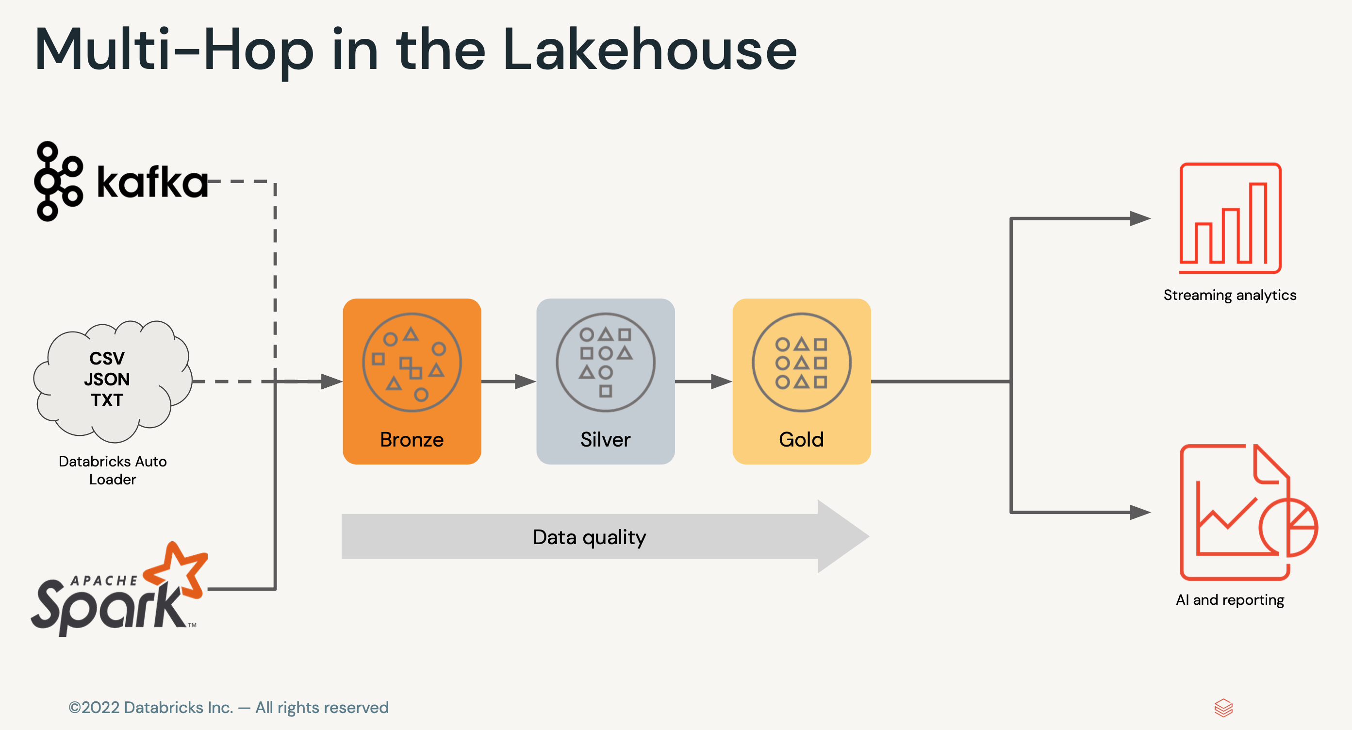
Bronze Layer (Raw Data)
- Append-only ingestion
- No business logic
- Schema minimally enforced
- Supports replay / backfill
Silver Layer (Cleansed and Conformed Data)
- Deduplication
- Joins / normalization
- Schema enforcement
- Basic data quality checks
Gold Layer (Curated Business-level tables)
- Business logic
- Aggregations
- KPI tables
- Semantic-ready datasets
                 (Many Inputs)
     Kafka     APIs     Files     DBs     Streams
        \        |        |        |        /
         \       |        |        |       /
          \      |        |        |      /
           \     |        |        |     /
            ▼    ▼        ▼        ▼    ▼

           ╔══════════════════════╗
           ║       BRONZE         ║   ← Wide ingest funnel
           ║  (Raw / Append-only)║
           ╚══════════════════════╝
                     │
                     │  (filter, dedupe, schema fix)
                     ▼
           ╔══════════════════════╗
           ║       SILVER         ║   ← Compression layer
           ║ (Clean / Conformed) ║
           ╚══════════════════════╝
                     │
                     │  (business logic, joins)
                     ▼
           ╔══════════════════════╗
           ║        GOLD          ║   ← High-value core
           ║ (Aggregated / KPI)  ║
           ╚══════════════════════╝
                     │
        ┌────────────┼────────────┬────────────┬────────────┐
        ▼            ▼            ▼            ▼            ▼

   BI / SQL     ML Features     APIs      Reverse ETL    Real-time Apps
 (Dashboards)   (Feature Store) (Serving)  (Salesforce)   (Streams)
Different Personas involved
- Data Engineer
- Data Analysts
- Data Scientists
#medallion #bronze #silver #gold
[Avg. reading time: 1 minute]
Data Quality Checks
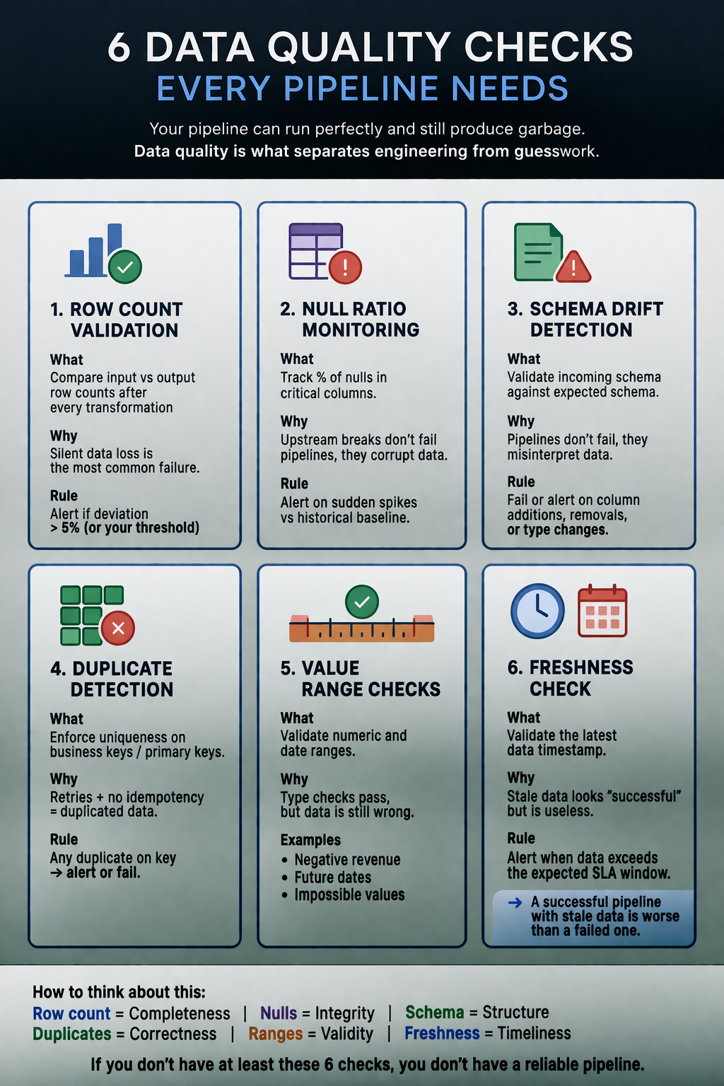
#dataquality #validation #schemadrift
[Avg. reading time: 3 minutes]
Data Engineering Model
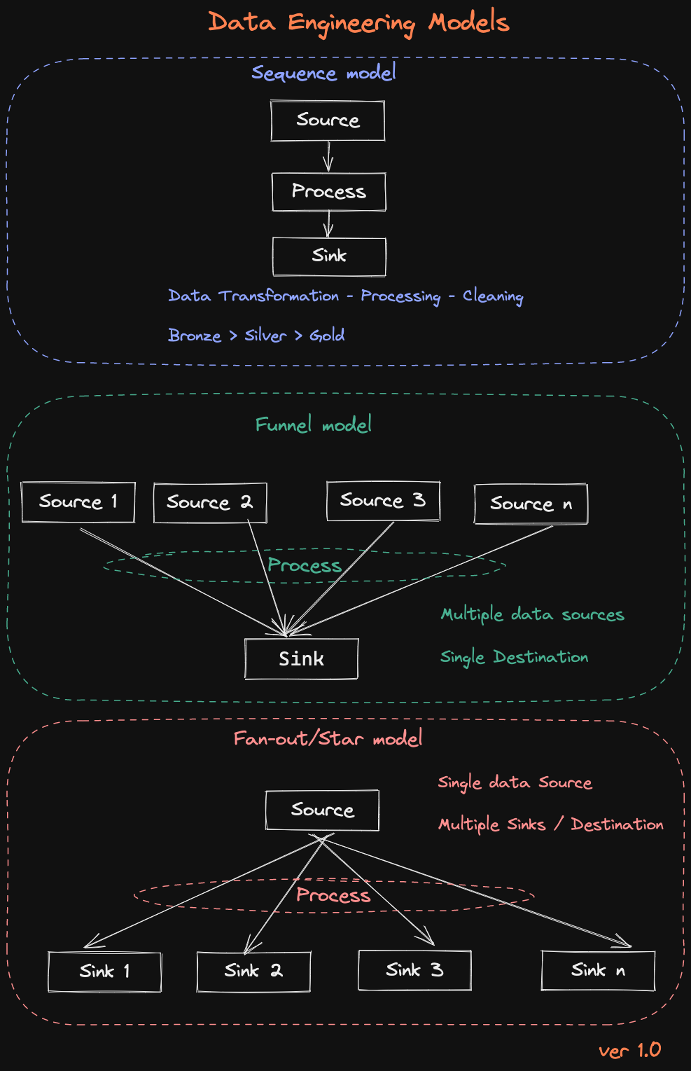
1. Sequence Model
Source > Process > Sink
This is the simplest and most common pattern.
- Data flows in a straight line
- Each step transforms the data
- Typically implemented as Bronze → Silver → Gold
Where it fits
- ETL pipelines
- Batch processing
- Data cleaning and enrichment
Example
Raw logs > cleaned logs > aggregated reports
Funnel Model
Multiple Sources > Process > Single Sink
Here, multiple inputs are combined into one destination.
- Data from different systems is merged
- Requires schema alignment and joins
- Often introduces data quality challenges
Where it fits
- Data warehouse ingestion
- Building unified datasets
- Customer 360 views
Example
CRM + Transactions + Web logs → Unified customer table
Fan-Out (Star) Model
Single Source > Process > Multiple Sinks
One dataset feeds multiple downstream consumers.
- Same data used in different ways
- Different outputs for different use cases
- Requires careful data contracts
Where it fits
- Serving layer
- Analytics + ML + APIs from same data
- Reverse ETL
Example
Gold table > BI dashboards + ML models + APIs
[Avg. reading time: 5 minutes]
Data Quality & Governance
Data Quality is simple
Can you trust this data to make a decision?
If not, it’s useless.
What matters
- Accuracy : Is it correct?
- Completeness : Is anything important missing?
- Consistency : Does it match across systems?
- Timeliness : Is it fresh or stale?
- Relevance : Do we even need this data?
How you improve it (practical, not theory)
- Profile data : find issues early
- Validate at entry : stop bad data upfront
- Clean regularly : fix what slipped through
- Track metrics : monitor trends over time
- Standardize core data (MDM) : one version of truth
Data Governance (Who controls the data)
Data governance is not a document.
It’s control.
Who owns data, who can use it, and how it’s protected.
What it includes
- Policies : rules for storing and sharing data
- Ownership : someone accountable (data stewards)
- Security : who can access what
- Compliance : laws you cannot ignore
- Metadata : context (where data came from, how to use it)
Laws you can’t ignore
You don’t need to memorize all of them.
Just understand the pattern: protect user data or pay heavily.
- GDPR (EU) : strictest, global impact
- CCPA (California) : consumer rights
- HIPAA (US) : healthcare data
GDPR (the one everyone cares about)
- Consent : you must ask clearly
- Access : users can see their data
- Delete : users can ask to remove it
- Portability : users can take their data
- Breach reporting : within 72 hours
- Fines : up to 4% of global revenue
Summary
- Data Quality = Is the data good?
- Data Governance = Are we allowed to use it?
[Avg. reading time: 7 minutes]
Data Mesh
What it is
Data Mesh is not a tool.
It’s a way to organize data ownership in large organizations.
Instead of one central data team owning everything,
each domain owns its own data.
- Finance owns finance data
- Sales owns sales data
- Marketing owns marketing data
Why it exists
Centralized data platforms don’t scale well.
Problems you see:
- One team becomes a bottleneck
- No clear ownership
- Slow delivery
- Constant dependency on data engineers
Data Mesh tries to fix this.
Before vs After
Monolithic Data Platform
- Central team owns everything
- Pipelines become complex and slow
- No clear ownership
- Everyone depends on one team
Data Mesh
- Data is split by domain
- Each team owns their pipelines
- Faster development
- Clear accountability
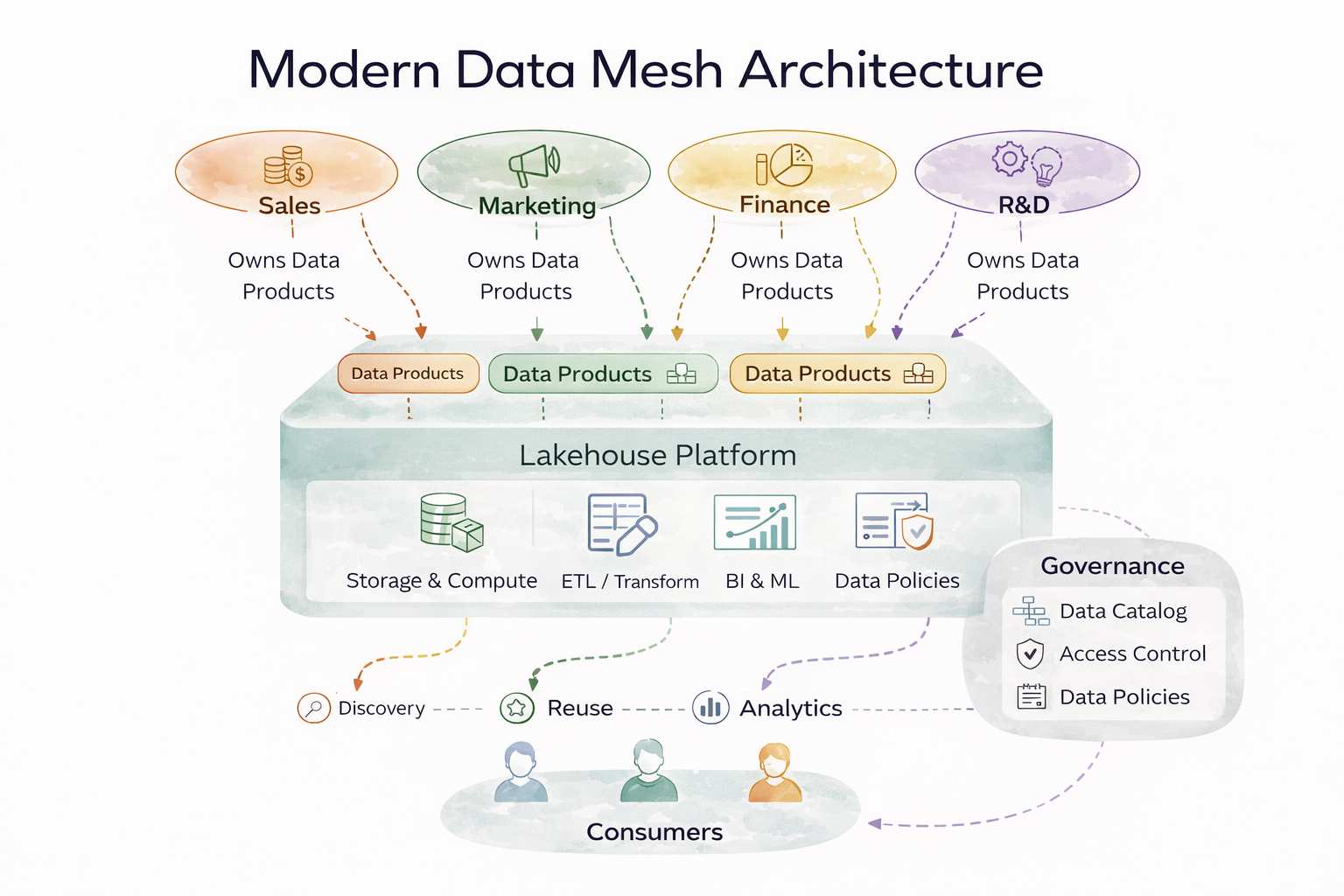
4 Core Principles
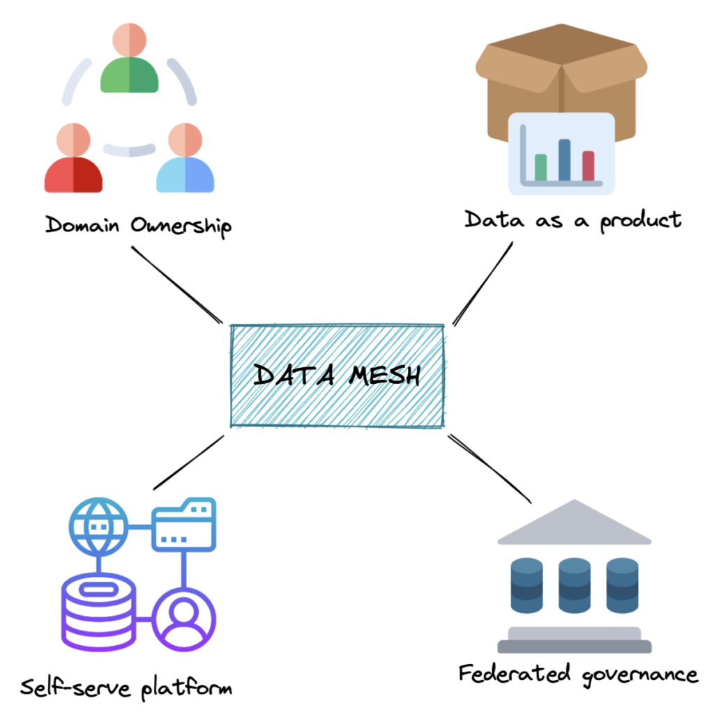
1. Domain Ownership
Each domain team owns:
- Data
- Pipelines
- Quality
You build it, you own it
2. Data as a Product
Data is not just tables.
It must be:
- Discoverable
- Reliable
- Documented
- Easy to use
If nobody can use your data, it’s useless
3. Self-Service Platform
Central team still exists.
But they provide:
- Infrastructure
- Tools
- Standards
Platform team builds the road, domains drive on it
4. Federated Governance
- Global rules (security, compliance)
- Local ownership (domains decide implementation)
Balance control and flexibility
Data Products
A data product is more than a dataset.
It includes:
- Data
- Metadata
- Documentation
- Code / pipelines
- SLAs
Treat data like a product, not a byproduct
Where Data Mesh works well
- Large organizations
- Many independent teams
- High data ownership conflicts
Where it fails
- Small teams (overkill)
- Weak engineering culture
- No governance discipline
- No platform team
Challenges
- Cross-domain joins become painful
- Standards drift across teams
- Requires strong ownership mindset
- More roles - more coordination
- Expensive to implement
Data Mesh is rarely implemented fully.
What most companies do
Most companies do is a Hybrid model
- Central platform (Example: Fabric, Databricks, Snowflake)
-
- Domain ownership (partial Mesh)
To get access to lots of external data.
#datamesh #domainownership #selfservice
1: https://www.dremio.com/resources/guides/what-is-a-data-mesh/
[Avg. reading time: 1 minute]
KAFKA
[Avg. reading time: 11 minutes]
Apache Kafka — Introduction
What Problem Does Kafka Solve?
When systems need to handle millions of events per second reliably, traditional messaging systems start failing.
- Data loss
- Poor scalability
- No easy replay of events
Kafka is built to solve these problems.
What is Kafka?
Apache Kafka is a distributed event streaming platform designed for:
- High throughput
- Fault tolerance
- Real-time data pipelines
At its core, Kafka is:
- A distributed commit log
- A publish-subscribe system
- A replayable event store
Key Characteristics
- High Throughput → Millions of messages per second
- Scalable → Horizontally scalable across brokers
- Fault-Tolerant → Data replication across servers
- Durable → Messages persisted and replayable
How Kafka Works
- Producer sends a message
- Kafka assigns it to a partition
- Message gets an offset
- Stored in a broker
- Consumers read using offsets
Basic Terms
1. Producer
A producer sends data to Kafka.
- Publishes messages to topics
- Can:
- Send to a specific partition
- Let Kafka decide
Partitioning logic:
- With key →
hash(key) % partitions - Without key → round-robin
2. Topic
A topic is a logical stream where messages are stored.
- Similar to a table or data stream
- Supports multiple consumers
- Append-only (no updates/deletes)
3. Message (Record)
A message is the basic unit of data in Kafka.
Structure:
- Key (optional) → partitioning
- Value → actual data
- Timestamp
- Headers (optional)
Messages are immutable.
4. Key
The key determines how messages are distributed.
- Same key → same partition
- Maintains ordering per key
If no key:
- Kafka uses round-robin distribution
5. Partition
A partition is a subset of a topic.
- Enables parallelism and scalability
- Append-only and ordered
Important:
- Each message has an offset
- Ordering is guaranteed only within a partition
- No global ordering across topic
6. Broker
A broker is a Kafka server.
Responsibilities:
- Receives messages
- Stores partitions
- Serves consumers
7. Consumer
A consumer reads messages from topics.
- Pull-based model
- Reads using offsets
- Can replay data
8. Consumer Group
A consumer group is a set of consumers working together.
- Each partition → only ONE consumer in group
- Enables parallel processing
Rebalancing:
- Happens when consumers join/leave
- Kafka redistributes partitions
9. Offset
An offset is a unique ID for messages in a partition.
- Starts from 0
- Incremental and immutable
Types:
- Current Offset → next to read
- Committed Offset → last saved
Kafka stores offsets in: __consumer_offsets
10. Batches
A batch is a group of messages sent together.
Benefits:
- Better network usage
- Compression
- Faster I/O
Trade-off:
- Larger batch → higher latency
- Smaller batch → lower latency
Brokers, Cluster, and Replication
Broker
- Single Kafka server
- Stores partitions
Cluster
- Multiple brokers working together
- Provides scalability and fault tolerance
Replication
- Partitions are replicated across brokers
- Ensures durability and availability
Message Delivery Semantics
Kafka supports three delivery guarantees:
1. At Most Once
- No duplicates
- Possible data loss
2. At Least Once (Default)
- No data loss
- Possible duplicates
3. Exactly Once
- No duplicates
- No data loss
- Higher overhead
- At Most Once → Fast but risky
- At Least Once → Safe but duplicates
- Exactly Once → Correct but expensive
Commit Strategies
-
Auto Commit
- Automatic at intervals
-
Manual Commit
- Controlled by consumer
- More reliable
Real-World Use Cases
- Log aggregation
- Event-driven microservices
- Real-time analytics
- Fraud detection
- User activity tracking
Summary
Kafka is not just a message queue.
It is a:
- Distributed log
- Streaming backbone
- Real-time data platform
Use Kafka when:
- Scale matters
- Reliability matters
- Real-time processing matters
[Avg. reading time: 3 minutes]
Kafka Use Cases
Data Streaming
Kafka can stream data in real time from various sources, such as sensors, applications, and databases. This data can then be processed and analyzed in real-time or stored for later analysis.
Log Aggregation
Kafka can be used to aggregate logs from various sources. This can help improve system logs’ visibility and facilitate troubleshooting.
Message Queuing
Kafka can decouple applications and services as a message queue. This can help to improve the scalability and performance of applications.
Web Activity Tracking
Kafka can track web activity in real-time. This data can then be used to analyze user behavior and improve the user experience.
Data replication
Kafka can be used to replicate data between different systems. This can help to ensure that data is always available and that it is consistent across systems.
[Avg. reading time: 10 minutes]
Kafka Software
2: Using Docker
Step 1
mkdir kafka-demo
cd kafka-demmo
Step 2
create a new file docker-compose.yml
services:
  kafka:
    image: docker.io/apache/kafka
    container_name: kafka
    ports:
      - "9092:9092"
      - "9093:9093"
    environment:
      - KAFKA_KRAFT_MODE=true
      - KAFKA_CFG_NODE_ID=1
      - KAFKA_CFG_PROCESS_ROLES=broker,controller
      - KAFKA_CFG_CONTROLLER_QUORUM_VOTERS=1@kafka:9093
      - KAFKA_CFG_CONTROLLER_LISTENER_NAMES=CONTROLLER
      - KAFKA_CFG_LISTENERS=PLAINTEXT://:9092,CONTROLLER://:9093
      - KAFKA_CFG_ADVERTISED_LISTENERS=PLAINTEXT://localhost:9092
      - KAFKA_CFG_LISTENER_SECURITY_PROTOCOL_MAP=PLAINTEXT:PLAINTEXT,CONTROLLER:PLAINTEXT
      - ALLOW_PLAINTEXT_LISTENER=yes
      - KAFKA_CFG_AUTO_CREATE_TOPICS_ENABLE=true
      - KAFKA_CFG_NUM_PARTITIONS=3
      - KAFKA_CFG_DEFAULT_REPLICATION_FACTOR=1
    volumes:
      - kafka_data:/bitnami/kafka

volumes:
  kafka_data:
    driver: local
Step 3
docker compose up -d
Step 4
Verification
docker container ls
Check the logs
docker logs kafka
Step 5: Create a new Kafka Topic
docker exec -it kafka kafka-topics.sh \
  --create \
  --topic gctopic \
  --bootstrap-server localhost:9092 \
  --partitions 3 \
  --replication-factor 1
Step 6: Producer
docker exec -it kafka kafka-console-producer.sh \
--topic gctopic \
--bootstrap-server localhost:9092 \
--property "parse.key=true" \
--property "key.separator=:"
Step 7: Consumer (Terminal 1)
docker exec -it kafka kafka-console-consumer.sh \
  --topic gctopic \
  --bootstrap-server localhost:9092 \
  --group 123 \
  --property print.partition=true \
  --property print.key=true \
  --property print.timestamp=true \
  --property print.offset=true
Consumer (Terminal 2)
docker exec -it kafka kafka-console-consumer.sh \
  --topic gctopic \
  --bootstrap-server localhost:9092 \
  --group 123 \
  --property print.partition=true \
  --property print.key=true \
  --property print.timestamp=true \
  --property print.offset=true
Consumer (Terminal 3)
docker exec -it kafka kafka-console-consumer.sh \
  --topic gctopic \
  --bootstrap-server localhost:9092 \
  --group 123 \
  --property print.partition=true \
  --property print.key=true \
  --property print.timestamp=true \
  --property print.offset=true
Consumer (Terminal 4)
This “new group” will receive all the messages published across partitions.
docker exec -it kafka kafka-console-consumer.sh \
  --topic gctopic \
  --bootstrap-server localhost:9092 \
  --group 456 \
  --property print.partition=true \
  --property print.key=true \
  --property print.timestamp=true \
  --property print.offset=true
Kafka messages can be produced and consumed in many ways.
- JAVA
- Python
- Go
- CLI
- REST API
- Spark
and so on..
Similar tools
Amazon Kinesis
A cloud-based service from AWS for real-time data processing over large, distributed data streams. Kinesis is often compared to Kafka but is managed, making it easier to set up and operate at scale. It’s tightly integrated with the AWS ecosystem.
Microsoft Event Hubs
A highly scalable data streaming platform and event ingestion service, part of the Azure ecosystem. It can receive and process millions of events per second, making it suitable for big data scenarios.
Google Pub/Sub
A scalable, managed, real-time messaging service that allows messages to be exchanged between applications. Like Kinesis, it’s a cloud-native solution that offers durable message storage and real-time message delivery without the need to manage the underlying infrastructure.
RabbitMQ
A popular open-source message broker that supports multiple messaging protocols. It’s designed for scenarios requiring complex routing, message queuing, and delivery confirmations. It’s known for its simplicity and ease of use but is more traditionally suited for message queuing rather than log streaming.
#kafka #softwares #kinesis #pubsub
[Avg. reading time: 0 minutes]
Python Scripts
Steps
Fork and Clone the repository.
git clone https://github.com/gchandra10/python_kafka_3_node_demos.git
uv sync
[Avg. reading time: 5 minutes]
Types of Streaming
Stateless Streaming
- Processes each record independently
- No memory of previous events
- Simple transformations and filtering
- Highly scalable
Examples of Stateless
- Unit conversion (Celsius to Fahrenheit) for each reading
- Data validation (checking if temperature is within realistic range)
- Simple transformations (rounding values)
- Filtering (removing invalid readings)
- Basic alerting (if current temperature exceeds threshold)
Use Cases:
- You only need to process current readings
- Simple transformations are sufficient
- Horizontal scaling is important
- Memory resources are limited
Stateful Streaming:
- Maintains state across events
- Enables complex processing like windowing and aggregations
- Requires state management strategies
- Good for pattern detection and trend analysis
Examples of Stateful
- Calculating moving averages of temperature
- Detecting temperature trends over time
- Computing daily min/max temperatures
- Identifying temperature patterns
- Calculating rate of temperature change
- Detecting anomalies based on historical patterns
- Unusual suspicious financial activity
Use Cases:
- You need historical context
- Analyzing patterns or trends
- Computing moving averages
- Detecting anomalies
- Time-window based analysis is required
Different Ingestion Services
Stream Processing Frameworks:
Structured Streaming (Apache Spark)
A processing framework for handling streaming data Part of Apache Spark ecosystem
Message Brokers/Event Streaming Platforms:
Apache Kafka (Open Source)
- Distributed event streaming platform
- Self-managed
Amazon MSK
- Managed Kafka service
- AWS managed version of Kafka
Amazon Kinesis
- AWS native streaming service
- Different from Kafka-based solutions
Azure Event Hubs
- Cloud-native event streaming service
- Azure’s equivalent to Kafka
#kinesis #stateful #stateless #eventhubs
[Avg. reading time: 1 minute]
Cloud Computing
- Introduction
- Types of Cloud Services
- Challenges
- Multi-Cloud
- High Availability
- Disaster Recovery (DR)
- RTO - RPO
- Cloud Native vs Lift-and-Shift
- Azure Cloud
[Avg. reading time: 6 minutes]
Introduction to Cloud Computing
Definitions
- Hardware: Physical computing components such as servers, storage devices, and networking equipment
- Software: Programs and systems such as operating systems, Microsoft Word, and Excel
- Website: Read-only web content (e.g., company pages, portfolios, news sites)
- Web Application: Interactive, read-write platforms (e.g., Google Docs, email, online forms)
What is Cloud Computing?
Cloud computing plays a critical role in the Big Data ecosystem.
Modern organizations deal with continuously growing data in terms of size, speed, and complexity. Cloud enables them to handle this efficiently without owning physical infrastructure.
- Cloud Computing: On-demand delivery of IT resources over the internet with a pay-as-you-go pricing model
Key Perspective
Cloud is often misunderstood because different teams interact with different layers:
- Compute (VMs, containers)
- Storage (object, block)
- Networking
- IAM (Identity and Access Management)
- Managed services
Each team sees only a slice and assumes that is the cloud.

- Cloud is not just servers or storage
- It is an abstraction layer over distributed systems
Shared responsibility is the core operating principle of cloud computing
Big Data Characteristics (6 V’s)
- Volume: Amount of data
- Velocity: Speed of data generation and processing
- Variety: Different data types (structured, semi-structured, unstructured)
- Veracity: Data quality and reliability
- Value: Business usefulness
- Vulnerability: Security and privacy risks
Cloud platforms help manage all these dimensions in an integrated way.
Why Cloud for Big Data?
- Cost savings (no upfront infrastructure)
- Scalability and flexibility
- High availability and reliability
- Built-in security controls
- Faster insights using managed analytics tools
- Collaboration across distributed teams
- Disaster recovery and backup
- Automatic updates and maintenance
Types of Cloud Computing
Public Cloud
- Owned and operated by third-party providers
- Examples: AWS, Azure, GCP
Private Cloud
- Dedicated infrastructure for a single organization
- Greater control, higher cost
Hybrid Cloud
- Combination of public and private cloud
- Enables workload portability and better control over sensitive data
[Avg. reading time: 15 minutes]
Types of Cloud Services
SaaS: Software as a Service
SaaS delivers ready-to-use software applications over the internet. Users do not manage the infrastructure, platform, or most application settings.
Examples:
- Google Workspace
- Dropbox
- Slack
- Salesforce
Key Characteristics
- Accessed through a web browser or thin client
- Managed centrally by the provider
- Usually follows a multi-tenant model
- Updates and patches are handled by the provider
- Minimal setup and maintenance for users
When Not to Use SaaS
- Limited or unreliable internet access
- Mission-critical workloads with very low downtime tolerance
- Applications requiring deep customization
- Tight integration with specialized on-premise hardware
- Strict data residency or regulatory constraints
- Performance-sensitive workloads that depend on local execution
PaaS: Platform as a Service
PaaS provides a managed environment for building, deploying, and running applications without requiring users to manage the underlying infrastructure.
Examples:
- Heroku
- Streamlit
- PythonAnywhere
Key Characteristics
- Developers focus on application code, not infrastructure
- Built-in support for deployment, scaling, and monitoring
- Provider manages runtime, middleware, patches, and much of the operations work
- Speeds up development and release cycles
- Often integrates well with CI/CD pipelines
When Not to Use PaaS
- Risk of vendor lock-in
- Limited control over infrastructure and runtime configuration
- Specialized compliance or security requirements
- Need for unsupported languages, frameworks, or custom system dependencies
- Performance-sensitive workloads needing low-level tuning
- Applications tightly coupled with legacy systems or custom middleware
IaaS: Infrastructure as a Service
IaaS provides virtualized compute, storage, and networking resources over the internet. Users manage the operating systems, middleware, and applications, while the provider manages the physical hardware.
Examples:
- Amazon EC2
- Google Compute Engine
- Microsoft Azure Virtual Machines
Key Characteristics
- High flexibility and control
- Resources can scale up or down based on demand
- Pay-as-you-go pricing
- Suitable for lift-and-shift migrations
- Supports custom operating systems and software stacks
When Not to Use IaaS
- High operational complexity
- Teams lack infrastructure expertise
- Ongoing maintenance overhead for OS, patches, and security
- Predictable workloads that may be cheaper or simpler on other models
- High availability and disaster recovery require careful design
- Compliance and security responsibilities remain heavily on the user
DBaaS: Database as a Service
DBaaS provides a fully managed database in the cloud. The provider handles infrastructure, provisioning, patching, backups, scaling, and high availability, while users focus on storing, querying, and managing data.
Examples:
- Neon (PostgreSQL)
- Amazon RDS
- Google Cloud SQL
- Azure SQL Database
- ClickHouse Cloud
Key Characteristics
- Managed database infrastructure
- Automated backups and recovery
- Built-in scaling and replication options
- Reduced operational overhead
- Users focus on schema, queries, and data access
When Not to Use DBaaS
- Need deep control over database internals or host OS
- Strict latency requirements with on-premise systems
- Regulatory or data residency constraints
- Very specialized database tuning or custom extensions
- Workloads where self-managed databases are more cost-effective at scale
Easy Way to Remember
- PaaS: deploy your application
- DBaaS: use a managed database for your application
Comparison between Services
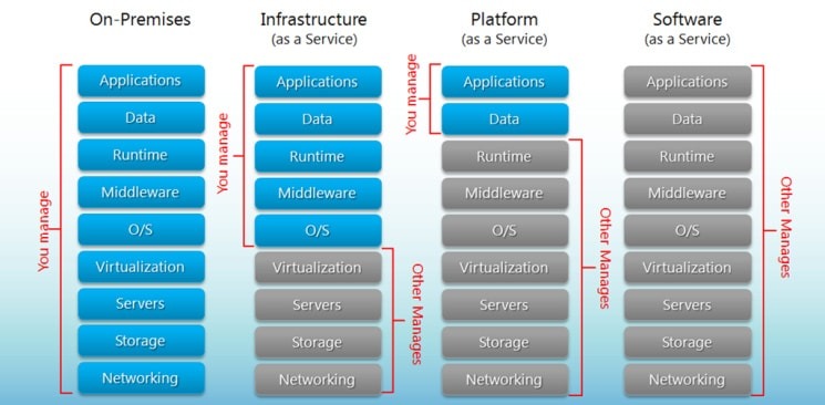
FaaS: Function as a Service
FaaS, often associated with serverless computing, lets developers run event-driven functions without managing servers. The cloud provider handles provisioning, scaling, and infrastructure maintenance.
Examples:
- AWS Lambda
- Azure Functions
- Google Cloud Functions
Key Characteristics
- Event-driven execution
- Automatic scaling
- Pay only for execution time and resources consumed
- No server provisioning or management
- Well suited for lightweight, modular workloads
When Not to Use FaaS
- Long-running tasks
- Complex stateful workflows
- Latency-sensitive applications affected by cold starts
- Heavy compute-intensive jobs
- Strong dependence on provider-specific services
- Constant, predictable workloads where containers or VMs may be more efficient
Quick Comparison
| Model | What You Manage | What Provider Manages | Best For |
|---|---|---|---|
| SaaS | Minimal user settings and usage | Application, platform, infrastructure | End-user software |
| PaaS | Application code and data | Infrastructure, OS, runtime, middleware | App development and deployment |
| IaaS | OS, middleware, apps, data | Physical hardware, virtualization | Maximum control and flexibility |
| FaaS | Function code and logic | Infrastructure, scaling, execution environment | Event-driven, serverless workloads |
Easy way to remember SaaS, PaaS, IaaS
- SaaS: Use the software
- PaaS: Build the software
- IaaS: Manage the software and OS on rented infrastructure
- FaaS: Run small functions without managing servers
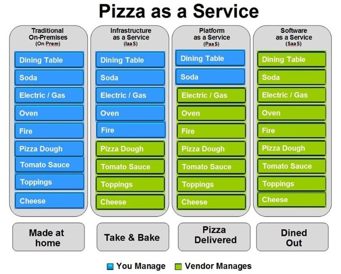
#saas #iaas #paas #faas #dbaas
1: src: http://bigcommerce.com
[Avg. reading time: 3 minutes]
Challenges of Cloud Computing
Privacy
- Sensitive data (PII, financial, health) lives in the cloud
- Requires strong controls: encryption, IAM, audits
- Breaches = high impact + regulatory exposure
Compliance
- Data replication across regions can violate data residency laws
- Regulations may restrict where data is stored/processed
- Example: Google Cloud Platform (GCP) lacks mainland China regions
Data Availability
- Depends on network + provider reliability
- Major providers (AWS, Azure, GCP) offer redundancy
- Still vulnerable to outages and regional failures
Connectivity
- Internet quality directly impacts performance
- High latency or downtime affects apps and pipelines
Vendor Lock-In
- Proprietary APIs/services make migration costly
- Rewrites and data movement add friction
Data Transfer Costs
- Egress (data leaving cloud) is expensive
- Large-scale pipelines can silently drive costs up
Limited Control
- No access to underlying infrastructure
- Less flexibility for tuning, customization, and debugging
[Avg. reading time: 9 minutes]
Multi-Cloud
Popular Cloud Providers
-
Amazon Web Services (AWS)
Market leader with the broadest range of services. Strong in compute, storage, and global infrastructure. -
Microsoft Azure
Widely used in enterprises due to tight integration with Microsoft products like Windows Server, Active Directory, and Office. -
Google Cloud Platform (GCP)
Strong in data analytics, big data processing, and machine learning (e.g., BigQuery). -
IBM Cloud
Focused on hybrid cloud and enterprise-grade solutions. -
Oracle Cloud (OCI)
Known for database services and enterprise workloads.
What is Multi-Cloud?
Multi-cloud is an approach where an organization uses multiple cloud providers instead of relying on a single one.
Example:
- AWS for infrastructure
- GCP for analytics
- Azure for enterprise applications
Why Multi-Cloud is Needed
-
Avoid Vendor Lock-in
Prevents dependency on a single provider’s pricing, tools, and limitations. -
Best-of-Breed Services
Different providers excel in different areas:- AWS : infrastructure maturity
- GCP : analytics and AI
- Azure : enterprise integration
-
Improved Reliability
Reduces risk of total system failure if one provider experiences an outage. -
Regulatory Requirements
Some workloads must run in specific regions or environments, requiring multiple providers.
Limitations of Single Cloud
-
Vendor Lock-in
Migration becomes difficult once deeply integrated with one provider. -
Pricing Constraints
No negotiation power if fully dependent on one vendor. -
Service Gaps
No single provider is best at everything. -
Single Point of Failure
Outages in one cloud can impact the entire system.
Ingress vs Egress
-
Ingress
Data entering the cloud.
Typically free of cost. -
Egress
Data leaving the cloud.
Typically charged, and often expensive.
Why it matters:
- Moving data between clouds incurs egress costs
- Example: Transferring data from AWS to GCP → AWS charges egress fees
Cloud Cost Considerations
-
Compute Costs
Charges for virtual machines, containers, and serverless functions. Usually predictable. -
Storage Costs
Low per unit, but grows significantly with scale. -
Data Transfer Costs (Egress)
Often the hidden cost driver, especially in multi-cloud setups. -
Managed Services Premium
Higher cost for convenience (managed databases, AI services, etc.) -
Idle Resources
Unused or overprovisioned resources can significantly increase costs.
Challenges of Multi-Cloud
-
Operational Complexity
Different tools, APIs, and configurations across providers. -
Skill Requirements
Teams must understand multiple cloud ecosystems. -
Data Movement Costs
Egress charges increase when transferring data between clouds. -
Monitoring and Management
Observability becomes more complex across platforms.
When to Use Multi-Cloud
- Need for high resilience across providers
- Advanced data and AI workloads
- Compliance or regulatory constraints
- Organizations with mature cloud teams
Summary
Multi-cloud provides flexibility, resilience, and access to best-in-class services, but it also introduces significant complexity and cost. It should be adopted only when there is a clear architectural or business need.
#aws #azure #oracle #gcp #multicloud
[Avg. reading time: 6 minutes]
High Availability
High Availability (HA) refers to designing systems that remain operational with minimal downtime over a given period.
It is often associated with uptime, but they are not the same:
- Uptime = observed system availability
- High Availability = design approach used to achieve high uptime
Availability Formula
- Availability = (Total Time - Downtime) / Total Time
This formula is used in SLAs and monitoring systems to measure system reliability.
Availability Levels and Downtime
Each additional “9” reduces downtime exponentially, not linearly.
99% Availability (Two Nines)
- Downtime: ~3.65 days per year
- Monthly Downtime: ~7.2 hours
- Suitable for non-critical systems
99.9% Availability (Three Nines)
- Downtime: ~8.76 hours per year
- Monthly Downtime: ~43.8 minutes
- Suitable for most business applications
99.99% Availability (Four Nines)
- Downtime: ~52.6 minutes per year
- Monthly Downtime: ~4.38 minutes
- Used for critical systems
99.999% Availability (Five Nines)
- Downtime: ~5.26 minutes per year
- Monthly Downtime: ~26.3 seconds
- Required for highly critical systems (finance, healthcare, telecom)
Why Each “9” Matters
- 99% → downtime in days
- 99.9% → downtime in hours
- 99.99% → downtime in minutes
- 99.999% → downtime in seconds
Each step requires significantly more advanced engineering and cost.
How High Availability is Achieved
- Redundancy (multiple servers or instances)
- Failover mechanisms (automatic switching)
- Load balancing
- No single point of failure
- Multi-region deployments
- Continuous monitoring and auto-recovery
SLA (Service Level Agreement)
- Availability is usually defined in SLAs
- Example: cloud providers like AWS, Azure, GCP offer ~99.9% to 99.99%
- If availability drops below SLA → customers receive service credits (not full compensation)
Cost of Downtime
- Average downtime cost: ~$5,600 per minute (Gartner estimate)
- Large enterprises can exceed $100,000 per minute
Higher availability reduces risk but increases infrastructure and operational costs.
Key Insight
- Moving from 99.9% → 99.99% is difficult
- Moving from 99.99% → 99.999% is extremely complex and expensive
High Availability is a trade-off between reliability, cost, and system complexity.
[Avg. reading time: 8 minutes]
Disaster Recovery (DR)
What is Disaster Recovery?
Disaster Recovery (DR) refers to the process of restoring systems, applications, and data after a failure or catastrophic event.
These events can include:
- Hardware failures
- Data center outages
- Cyberattacks (e.g., ransomware)
- Natural disasters (earthquakes, floods, fires)
Disaster Recovery vs High Availability (HA)
-
High Availability (HA)
Focuses on preventing downtime
Systems continue running with minimal or no interruption -
Disaster Recovery (DR)
Focuses on recovering after failure
Accepts downtime, but minimizes impact and recovery time
Simple way to think:
- HA = Avoid failure
- DR = Recover from failure
Why Disaster Recovery is Important
-
Business Continuity
Ensures operations can resume after unexpected failures -
Data Protection
Prevents permanent data loss -
Financial Impact Reduction
Downtime can cost thousands to millions per hour -
Compliance Requirements
Many industries require DR plans (finance, healthcare, etc.)
Types of Disaster Recovery Strategies
1. Backup and Restore
- Regular backups stored in another location
- Restore systems when failure occurs
Pros:
- Low cost
- Simple to implement
Cons:
- High recovery time
- Possible data loss
2. Pilot Light
- Minimal version of system always running in another region
- Scale up during disaster
Pros:
- Faster recovery than backup
- Lower cost than full duplication
Cons:
- Requires scaling during recovery
3. Warm Standby
- Fully functional but scaled-down system running in another region
Pros:
- Faster recovery
- Moderate cost
Cons:
- Still not instant failover
4. Active-Active (Multi-Region)
- Systems run simultaneously in multiple regions
Pros:
- Near-zero downtime
- High resilience
Cons:
- Very expensive
- Complex to manage
Key Concepts in Disaster Recovery
Backup Types
- Full Backup – Entire dataset
- Incremental Backup – Only changes since last backup
- Differential Backup – Changes since last full backup
Replication
-
Synchronous Replication
Data written to multiple locations at the same time
(low data loss, higher latency) -
Asynchronous Replication
Data replicated with delay
(faster, but risk of data loss)
Disaster Recovery in Cloud
Cloud platforms simplify DR through:
- Multi-region deployments
- Automated backups
- Managed replication services
- Infrastructure as Code (IaC) for quick recovery
Example:
- Primary system in one region
- Backup or standby system in another region
Common Challenges
- Cost vs Recovery Speed Tradeoff
- Testing DR Plans
- Many systems fail because DR is never tested
- Data Consistency Issues
- Complex Architecture
- Human Error during recovery
Best Practices
- Define clear RTO and RPO targets
- Automate backups and replication
- Use multiple regions
- Regularly test recovery plans
- Document procedures clearly
Summary
Disaster Recovery is not about avoiding failure-it is about being prepared to recover quickly and effectively when failure happens. A strong DR strategy ensures business continuity, protects data, and reduces the impact of unexpected disruptions.
[Avg. reading time: 8 minutes]
RTO vs RPO
What are RTO and RPO?
Recovery Time Objective (RTO)
RTO is the maximum acceptable time a system can be down after a failure.
- Focus: Time to recover
- Question it answers:
“How fast do we need to restore the system?”
Recovery Point Objective (RPO)
RPO is the maximum acceptable amount of data loss, measured in time.
- Focus: Data loss tolerance
- Question it answers:
“How much data can we afford to lose?”
Simple Example
-
RTO = 2 hours
→ System must be back online within 2 hours -
RPO = 15 minutes
→ You can only lose up to 15 minutes of data
Key Differences
| Aspect | RTO | RPO |
|---|---|---|
| Focus | Downtime | Data Loss |
| Measured In | Time (minutes/hours) | Time (minutes/hours) |
| Goal | Restore service quickly | Minimize data loss |
| Driven By | System recovery capability | Backup/replication strategy |
When to Use RTO vs RPO
Use RTO when:
- System availability is critical
- Downtime directly impacts revenue or operations
- Examples:
- Banking systems
- E-commerce platforms
- Real-time services
Use RPO when:
- Data accuracy and integrity are critical
- Data loss has serious consequences
- Examples:
- Financial transactions
- Healthcare records
- Order processing systems
How to Define RTO and RPO
Step 1: Identify Critical Systems
- Which systems must recover fastest?
- Which systems can tolerate downtime?
Step 2: Analyze Business Impact
- What is the cost of downtime?
- What is the cost of data loss?
Step 3: Assign Targets
| System Type | RTO | RPO |
|---|---|---|
| Payment System | Minutes | Near Zero |
| Internal Tools | Hours | 1–2 Hours |
| Analytics System | Hours/Day | Several Hours |
How to Achieve RTO and RPO
Improving RTO (Faster Recovery)
- Use failover systems
- Deploy across multiple regions
- Use automation (Infrastructure as Code)
- Maintain warm or active standby systems
Improving RPO (Less Data Loss)
- Frequent backups
- Real-time replication
- Use distributed databases
- Enable continuous data protection
Trade-Off: Cost vs Recovery
-
Lower RTO → Higher cost
(requires active systems, redundancy) -
Lower RPO → Higher cost
(requires frequent backups or real-time replication)
Example:
- RPO = 0 (no data loss) → requires synchronous replication → expensive
- RTO = near zero → requires active-active setup → very expensive
Common Mistakes
- Setting unrealistic RTO/RPO without infrastructure support
- Not aligning targets with business needs
- Not testing recovery procedures
- Assuming backups alone are enough
Key Takeaway
- RTO = How fast you recover
- RPO = How much data you lose
Both must be defined together to design an effective disaster recovery strategy. Optimizing them always involves a trade-off between cost, complexity, and business requirements.
[Avg. reading time: 11 minutes]
Cloud Native vs Lift-and-Shift
Introduction
Organizations moving to the cloud typically follow one of two approaches:
- Cloud Native → Build or redesign applications specifically for the cloud
- Lift-and-Shift (Rehosting) → Move existing applications to the cloud with minimal or no changes
These approaches differ significantly in terms of architecture, cost, scalability, and long-term value.
What is Lift-and-Shift?
Lift-and-shift is the process of migrating applications from on-premises to the cloud without modifying their architecture.
Key Characteristics
- Minimal or no code changes
- Same architecture as on-premises
- Faster migration
- Uses virtual machines (VMs)
Example
-
Moving a legacy Java application from a local data center to a cloud VM (e.g., AWS EC2)
-
Netflix early 2008-2009 moved their Monolithic application on prem to AWS as quick exit from failing Data Centers. Later redesigned with microservices.
What is Cloud Native?
Cloud native refers to designing and building applications specifically for cloud environments using modern architectural patterns.
Key Characteristics
- Microservices architecture
- Containers (Docker, Kubernetes)
- Serverless computing
- Auto-scaling and resilience built-in
Example
- A microservices-based application using containers, APIs, and managed cloud services
Key Differences
| Aspect | Lift-and-Shift | Cloud Native |
|---|---|---|
| Approach | Rehost existing apps | Build/redesign for cloud |
| Speed | Fast migration | Slower (requires redesign) |
| Cost (initial) | Low | Higher |
| Cost (long-term) | Higher | Optimized |
| Scalability | Limited | Highly scalable |
| Architecture | Monolithic | Microservices |
| Cloud Utilization | Low | High |
| Maintenance | High | Lower (managed services) |
Use Cases for Lift-and-Shift
-
Quick cloud migration
- Deadlines or data center shutdowns
-
Legacy applications
- Difficult or risky to refactor
-
Short-term strategy
- “Move first, optimize later”
-
Cost of redesign is too high
- When ROI of refactoring is unclear
Use Cases for Cloud Native
-
New applications
- Built from scratch for scalability
-
High-scale systems
- E-commerce, streaming platforms, SaaS
-
Rapid innovation
- Frequent deployments and updates
-
Modernization initiatives
- Breaking monoliths into microservices
Advantages and Disadvantages
Lift-and-Shift
Advantages:
- Fast and simple migration
- Lower upfront effort
- Minimal risk during transition
Disadvantages:
- Does not leverage cloud capabilities
- Higher long-term costs
- Limited scalability and flexibility
Cloud Native
Advantages:
- High scalability and resilience
- Better cost optimization over time
- Faster development and deployment cycles
Disadvantages:
- Requires redesign and expertise
- Higher initial investment
- Increased architectural complexity
When to Choose Each Approach
Choose Lift-and-Shift if:
- You need quick migration
- Application is stable and rarely updated
- Refactoring is too risky or expensive
Choose Cloud Native if:
- You need scalability and flexibility
- Building new applications
- Want to leverage full cloud benefits
- Long-term cost and performance matter
Hybrid Approach (Most Common in Reality)
Most organizations use a combination of both:
- Lift-and-shift for legacy systems
- Gradual refactoring into cloud-native architecture
This approach is often called:
- Lift, Shift, and Optimize
Common Mistakes
- Treating lift-and-shift as a final solution
- Overengineering cloud-native systems unnecessarily
- Ignoring cost implications of poor architecture
- Lack of skilled teams for cloud-native development
Key Takeaway
- Lift-and-Shift = Speed and simplicity
- Cloud Native = Scalability and long-term efficiency
The right choice depends on business goals, timelines, and technical maturity. Most organizations start with lift-and-shift and evolve toward cloud-native architectures over time.
[Avg. reading time: 8 minutes]
Azure Cloud
Azure is a cloud computing platform provided by Microsoft that delivers computing resources over the internet on a pay-as-you-go model.
Core Concepts
Servers
Individual physical or virtual machines that provide compute power.
Data Centers
Physical facilities that host servers along with networking, storage, and other infrastructure components.
Availability Zones (AZs)
Each Availability Zone consists of one or more data centers within a region.
- Designed for high availability
- Provide fault isolation
- Connected through low-latency networking
Even if one data center fails, services in other zones continue to operate.
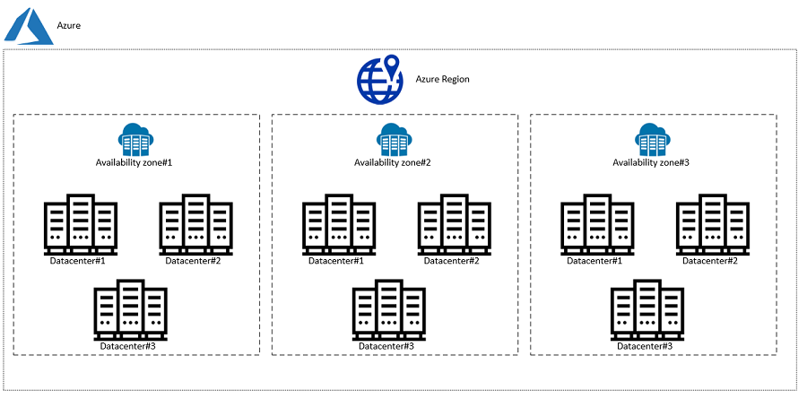
Source: https://www.unixarena.com/2020/08/what-is-the-availablity-zone-on-azure.html
Regions
Regions are geographically distinct locations that contain multiple Availability Zones.
- Help keep applications close to users
- Improve latency and performance
- Support data residency and compliance requirements
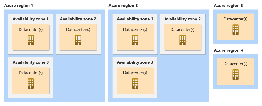
Source: https://learn.microsoft.com/en-us/azure/reliability/availability-zones-overview?tabs=azure-cli
Paired Regions
Azure regions are grouped into region pairs for disaster recovery.
- Located at least 300 miles apart
- Ensure isolation from large-scale failures
- Support cross-region replication
Geo-Redundant Storage (GRS)
- Data is stored in the primary region
- Automatically replicated to the paired secondary region
- Ensures durability and disaster recovery
Azure Site Recovery
Azure Site Recovery enables:
- Failover to a secondary region during outages
- Business continuity during disasters
- Automated recovery workflows
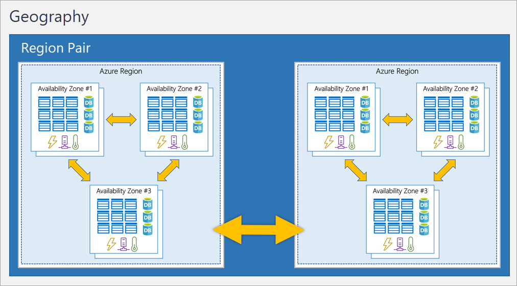
Source: https://i.stack.imgur.com/BwHct.png
How Everything Fits Together
- A Server runs your application
- Servers live inside a Data Center
- Multiple Data Centers form an Availability Zone
- Multiple Availability Zones form a Region
- Two Regions form a Paired Region
Real-World Example
Scenario: E-commerce Application
- Your application runs on servers in East US Region
- Deployed across 3 Availability Zones for high availability
- Database uses Geo-Redundant Storage (GRS)
- Backup region: West US (Paired Region)
What happens during failure?
- If one server fails : no impact
- If one data center fails : AZ handles it
- If entire region fails : failover to paired region
Minimal downtime, continuous service
Use Availability Zones when:
- You want high availability within a region
- Low latency is critical
Use Paired Regions when:
- You need disaster recovery
- You want protection from regional outages
Use Geo-Redundant Storage when:
- Data durability is more important than cost
Trade-offs
- Multi-zone deployments : Higher cost but better availability
- Multi-region deployments : Even higher cost + complexity
- GRS : More durable but increased storage cost and latency
[Avg. reading time: 5 minutes]
Azure Services
Azure cloud platform that helps you:
- Run applications
- Store data
- Connect systems
- Secure access
1. Compute (Run Applications)
Virtual Machines (VM)
- Cloud-based servers
- You manage OS and software
Use when:
- Full control is needed
- Running legacy applications
App Service
- Managed platform for web apps
- No server management
Use when:
- Hosting websites or APIs
Azure Functions
- Runs code only when triggered
Use when:
- Automation
- Background jobs
Containers / AKS
- Run containerized applications
Use when:
- Microservices
- Scalable systems
2. Storage (Store Data)
Blob Storage
- Stores files (images, videos, backups)
Data Lake Storage
- Optimized for big data and analytics
Azure Files
- Shared file storage
Use when:
- Lift-and-shift applications
3. Networking (Connect Systems)
Virtual Network (VNet)
- Private network in Azure
Load Balancer
- Distributes traffic across servers
Application Gateway
- Routes web traffic
- Includes Web Application Firewall (WAF)
ExpressRoute
- Private connection to Azure (no public internet)
4. Identity & Access (Security Basics)
Azure Active Directory (AAD)
- Manages users and login
RBAC (Role-Based Access Control)
- Controls who can access what
5. Monitoring & Management
Azure Monitor
- Tracks logs, metrics, and alerts
Azure Resource Manager (ARM)
- Used to deploy and manage resources
Azure Backup
- Backup and restore data
Azure Site Recovery
- Disaster recovery (failover to another region)
flowchart LR

User[User / Browser]

User -->|HTTPS| CDN[CDN / Front Door]
CDN --> AG[Application Gateway]

AG --> App[WebApp-App Service]

App --> API[Backend APIs]

API --> DB[(Database)]
API --> Cache[(Cache)]
API --> Storage[(Blob Storage)]

App --> Auth[Azure AD / Identity]

subgraph Azure Cloud
    CDN
    AG
    App
    API
    DB
    Cache
    Storage
    Auth
end
[Avg. reading time: 2 minutes]
How Do We Access Azure?
There are multiple ways to interact with Azure:
1. Azure Portal (Web UI)
- Browser-based interface
- Point-and-click experience
Use when:
- Learning Azure
- Exploring services
- Quick setup
2. Azure CLI
- Command-line tool (
azcommands) - Scriptable and fast
Example:
az group create --name myRG --location eastus
Use when:
- Automation
- Dev workflows
3. Azure PowerShell
- PowerShell-based commands
Use when:
- Windows admins
- Scripting in PowerShell
4. SDKs (Python, Java, etc.)
- Interact with Azure using code
Use when:
- Application integration
- Custom automation
Summary
- Portal → Manual
- CLI → Fast + Scriptable
- SDK → Programmable
[Avg. reading time: 6 minutes]
What is Infrastructure as Code
Infrastructure as Code (IaC) means:
Defining cloud resources using code instead of manually creating them.
Without IaC (Not best practice)
- Click in portal
- Create resources manually
- Hard to repeat
- Error-prone
With IaC (Best Practice)
- Write code to define resources
- Reusable and consistent
- Version controlled
Example (Conceptual)
Instead of:
- Manually creating VM
- Manually creating storage
You write code that says:
- Create 1 VM
- Create 1 Storage Account
- Connect them
IaC Tools in Azure
1. ARM Templates
- Native Azure JSON-based templates
2. Terraform
- Multi-cloud IaC tool
Why IaC Matters
- Repeatability : same setup every time
- Version Control : track changes
- Automation : faster deployments
- Reliability : fewer mistakes
Summary
- Deploy same setup multiple times
- Maintain consistency
- Automate environments (Dev / Test / Prod)
Azure Login
az login
Azure Group
az group list --output table

# Create a new Resource Group
az group create --name resgroup_via_cli --location eastus2

# delete the Resource Group
az group delete --name resgroup_via_cli

# Delete the Resource Group without Prompt
az group delete --name resgroup_via_cli -y

# List all VMs.

az vm list

# Azure List Sizes

az vm list-sizes --location eastus
Sample Basic VM
template.json
{
  "$schema": "https://schema.management.azure.com/schemas/2019-04-01/deploymentTemplate.json#",
  "contentVersion": "1.0.0.0",

  "parameters": {
    "vmName": { "type": "string", "defaultValue": "myVM" },
    "adminUsername": { "type": "string" },
    "adminPassword": { "type": "secureString" }
  },

  "resources": [
    {
      "type": "Microsoft.Compute/virtualMachines",
      "apiVersion": "2021-11-01",
      "name": "[parameters('vmName')]",
      "location": "[resourceGroup().location]",

      "properties": {
        "hardwareProfile": {
          "vmSize": "Standard_B1s"
        },

        "osProfile": {
          "computerName": "[parameters('vmName')]",
          "adminUsername": "[parameters('adminUsername')]",
          "adminPassword": "[parameters('adminPassword')]"
        },

        "storageProfile": {
          "imageReference": {
            "publisher": "Canonical",
            "offer": "UbuntuServer",
            "sku": "18_04-lts",
            "version": "latest"
          }
        }
      }
    }
  ]
}
Deploy ARM Template using Azure CLI
Step 1: Login to Azure
az login
Step 2: Create a Resource Group
az group create \
  --name myResourceGroup \
  --location eastus
Step 3: Deploy the ARM Template
az deployment group create \
  --resource-group myResourceGroup \
  --template-file template.json \
  --parameters adminUsername=azureuser adminPassword=YourPassword123
[Avg. reading time: 3 minutes]
IaC Concept: Idempotency
What is Idempotency?
Idempotency means:
Running the same code multiple times produces the same result.
Simple Example
If your code says:
- Create 1 Virtual Machine
Then:
- Run once : VM is created
- Run again : No duplicate VM
- Run again : Still only 1 VM
Why This Matters
Without idempotency:
- You might create duplicate resources
- Systems become inconsistent
- Hard to manage infrastructure
With Idempotency (IaC)
- Safe to run deployments multiple times
- Ensures desired state is maintained
- Prevents duplication
Real-World Analogy
Think of a light switch:
- Turn ON : light is on
- Turn ON again : still on (no change)
Same idea with infrastructure.
In Azure (ARM Templates)
- You define the desired state
- Azure checks current state
- Only applies necessary changes
IaC is not about “running commands”
It is about:
Declaring the final state and letting the system reach it
[Avg. reading time: 7 minutes]
Terraform
What is Terraform?
Terraform is a tool used to:
Define and manage cloud infrastructure using code
It works across multiple cloud providers like:
- Azure
- AWS
- Google Cloud
Why Terraform?
Instead of manually creating resources:
- Clicking in portal
- Running multiple commands
You write code once and Terraform:
- Creates everything
- Updates changes
- Keeps things consistent
Core Idea
You describe:
- What you want
Terraform figures out:
- How to create it
How Terraform Works
- Write configuration (code)
- Run
terraform plan: see what will happen - Run
terraform apply: create/update resources
How Idempotency works with Terraform
Terraform State
Terraform state is:
A file that keeps track of what Terraform has created
Terraform needs to know:
- What already exists
- What needs to change
- What to delete
Without state:
- Terraform would not know current infrastructure
- It could create duplicates or break things
Where is State Stored?
- Local file :
terraform.tfstate - Remote storage : Azure Storage, S3, etc.
Terraform does NOT check Azure directly every time.
It relies on:
State file as the source of truth
Terraform Example: Create a VM in Azure
Step 1: Install Terraform
Download from: https://developer.hashicorp.com/terraform/downloads
Verify:
terraform -version
Step 2: Create Project Folder
terraform-vm/
 ├── main.tf
Step 3: Write Terraform Code
Create main.tf:
provider "azurerm" {
  features {}
}

resource "azurerm_resource_group" "rg" {
  name     = "demo-rg"
  location = "East US"
}

resource "azurerm_virtual_network" "vnet" {
  name                = "demo-vnet"
  address_space       = ["10.0.0.0/16"]
  location            = azurerm_resource_group.rg.location
  resource_group_name = azurerm_resource_group.rg.name
}

resource "azurerm_subnet" "subnet" {
  name                 = "demo-subnet"
  resource_group_name  = azurerm_resource_group.rg.name
  virtual_network_name = azurerm_virtual_network.vnet.name
  address_prefixes     = ["10.0.1.0/24"]
}

resource "azurerm_network_interface" "nic" {
  name                = "demo-nic"
  location            = azurerm_resource_group.rg.location
  resource_group_name = azurerm_resource_group.rg.name

  ip_configuration {
    name                          = "internal"
    subnet_id                     = azurerm_subnet.subnet.id
    private_ip_address_allocation = "Dynamic"
  }
}

resource "azurerm_linux_virtual_machine" "vm" {
  name                = "demo-vm"
  resource_group_name = azurerm_resource_group.rg.name
  location            = azurerm_resource_group.rg.location
  size                = "Standard_B1s"
  admin_username      = "azureuser"

  network_interface_ids = [
    azurerm_network_interface.nic.id
  ]

  admin_password = "YourPassword123!"

  disable_password_authentication = false

  os_disk {
    caching              = "ReadWrite"
    storage_account_type = "Standard_LRS"
  }

  source_image_reference {
    publisher = "Canonical"
    offer     = "UbuntuServer"
    sku       = "18_04-lts"
    version   = "latest"
  }
}
Step 4: Login to Azure
az login
Step 5: Initialize Terraform
terraform init
Step 6: Preview Changes
terraform plan
Step 7: Apply (Create Resources)
terraform apply
Type:
yes
Step 8: Destroy Resources
terraform destroy
[Avg. reading time: 1 minute]
CLI Tools for Operational Efficiency
[Avg. reading time: 1 minute]
Introduction - CLI Tools
Knowlege of these tools are baseline skills required to function in real data engineering environments. This chapter focuses on command line proficiency, text processing, and direct manipulation of JSON and YAML using standard tools.
These skills are not tied to any single framework and apply across cloud platforms, data pipelines, and production systems.
[Avg. reading time: 1 minute]
Linux Commands - 01
The first set of Linux commands, so many websites to explain what these commands do or use your favourite AI tool.
MAC - Open Terminal
Windows - Open GIT BASH
hostname

whoami

uname

uname -a

ping

pwd

echo ""

mkdir <foldername>

cd <foldername>

touch <filename>

echo "sometext" > <filename>

cd ..  (space is needed)

ls [-l]

cp <filename> <filename1>
#linux #commands #cli #gitbash
[Avg. reading time: 1 minute]
Linux Commands - 02
The next set of Linux commands, so many websites to explain what these commands do or use your favourite AI tool.
wget

touch

echo

variables

|

cat

wc

more

head

tail

grep

cut

uniq

sort
[Avg. reading time: 5 minutes]
AWK
AWK is a scripting language used for manipulating data and generating reports. It’s a Domain Specific Language.
Demo Using AWK
wget
https://raw.githubusercontent.com/gchandra10/awk_scripts_data_science/master/sales_100.csv
Display file contents
awk '{print }' sales_100.csv
By default, AWK uses space as a delimiter. Since our file has a comma (,) let’s specify it with -F
awk -F ',' '{print }' sales_100.csv
To get the number of columns of each row, use the NF (a predefined variable)
awk -F ',' '{print NF}' sales_100.csv
AWK lets you choose specific columns.
awk -F ',' '{print $1,$2,$4}' sales_100.csv
Row Filter
AND = &&
OR = ||
Not = !
awk -F ',' '{if($4 == "Online") {print $1,$2,$4}}' sales_100.csv
awk -F ',' '{if($4 == "Online" && $5 =="L") {print $1,$2,$4,$5}}' sales_100.csv```
Variables
awk -F ',' '{sp=$9 * $10;cp=$9 * $11; {printf "%f,%f,%s,%s \n",sp,cp,$1,$2 }}' sales_100.csv
RegEx: Return all rows starting with A in Column 1
awk -F ',' '$1 ~ /^A/ {print}' sales_100.csv
Return all rows which have Space in Column 1
awk -F ',' '$1 ~ /\s/ {print}' sales_100.csv
AWK also has the functionality to change the column and row delimiter
OFS: Output Field Separator
ORS: Output Row Separator
awk -F ',' 'BEGIN{OFS="|";ORS="\n\n"} $1 ~ /^A/ {print substr($1,1,4),$2,$3,$4,$5}' sales_100.csv
Built-in Functions
awk -F ',' 'BEGIN{OFS="|";ORS="\n"} $1 ~ /^A/ {print tolower(substr($1,1,4)),tolower($2),$3,$4,$5}' sales_100.csv
[Avg. reading time: 3 minutes]
CSVSQL
SQL query on CSV file
Download CSV file to your local machine.
wget
https://raw.githubusercontent.com/gchandra10/awk_scripts_data_science/master/sales_100.csv
Simple query
csvsql --query "select * from sales_100" ./sales_100.csv
with Limit
csvsql --query "select * from sales_100 limit 5" ./sales_100.csv
using MAX aggregate function
csvsql --query "select max(unitprice) from sales_100 limit 5" ./sales_100.csv
Use double quotes to handle columns that have Space in between them in csvsql
csvsql --query 'select distinct("Order Priority") from sales_100' ./sales_100.csv
Using Group By
csvsql --query "select country,region,count(*) from sales_100 group by country, region" ./sales_100.csv
using WildCards
csvsql --query "select * from sales_100 where region like 'A%' order by region desc" sales_100.csv
[Avg. reading time: 8 minutes]
JQ
- jq is a lightweight and flexible command-line JSON processor.
- Reads JSON from stdin or a file, applies filters, and writes JSON to stdout.
- Useful when working with APIs, logs, or config files in JSON format.
- Handy tool in Automation.
- Download JQ CLI (Preferred) and learn JQ.
- Use the VSCode Extension and learn JQ.
Download the sample JSON
https://raw.githubusercontent.com/gchandra10/jqtutorial/refs/heads/master/sample_nows.json
Note: As this has no root element, '.' is used.
1. View JSON file in readable format
jq '.' sample_nows.json
2. Read the First JSON element / object
jq 'first(.[])' sample_nows.json
3. Read the Last JSON element
jq 'last(.[])' sample_nows.json
4. Read top 3 JSON elements
jq 'limit(3;.[])' sample_nows.json
5. Read 2nd & 3rd element. Remember, Python has the same format. LEFT Side inclusive, RIGHT Side exclusive
jq '.[2:4]' sample_nows.json
6. Extract individual values. | Pipeline the output
jq '.[] | [.balance,.age]' sample_nows.json
7. Extract individual values and do some calculations
jq '.[] | [.age, 65 - .age]' sample_nows.json
8. Return CSV from JSON
jq '.[] | [.company, .phone, .address] | @csv ' sample_nows.json
9. Return Tab Separated Values (TSV) from JSON
jq '.[] | [.company, .phone, .address] | @tsv ' sample_nows.json
10. Return with custom pipeline delimiter ( | )
jq '.[] | [.company, .phone, .address] | join("|")' sample_nows.json
Pro TIP : Export this result > output.txt and Import to db using bulk import tools like bcp, load data infile
11. Convert the number to string and return | delimited result
jq '.[] | [.balance,(.age | tostring)] | join("|") ' sample_nows.json
12. Process Array return Name (returns as list / array)
jq '.[] | [.friends[].name]' sample_nows.json
or (returns line by line)
jq '[].friends[].name' sample_nows.json
13. Parse multi level values
returns as list / array
jq '.[] | [.name.first, .name.last]' sample_nows.json
returns line by line
jq '.[].name.first, .[].name.last' sample_nows.json
14. Query values based on condition, say .index > 2
jq 'map(select(.index > 2))' sample_nows.json
jq 'map(select(.index > 2)) | .[] | [.index,.balance,.age]' sample_nows.json
15. Sorting Elements
# Sort by Age ASC
jq 'sort_by(.age)' sample_nows.json
# Sort by Age DESC
jq 'sort_by(-.age)' sample_nows.json
# Sort on multiple keys
jq 'sort_by(.age, .index)' sample_nows.json
Use Cases
curl -s https://www.githubstatus.com/api/v2/status.json
curl -s https://www.githubstatus.com/api/v2/status.json | jq '.'
curl -s https://www.githubstatus.com/api/v2/status.json | jq '.status'
#jq #tools #json #parser #cli #automation
[Avg. reading time: 1 minute]
YQ
YQ is a command line tool to read, query, transform, and write YAML
Its like jq for YAML. Written in Go, single binary, fast.
YAML files are popularly used in many tools, example: Kubernetes, Terraform, Github Actions.
YQ helps engineers to parse the YAML file and extract necessary output. The output can also be converted to JSON.
[Avg. reading time: 0 minutes]
Miscellaneous
[Avg. reading time: 5 minutes]
Additional Reading
Note 1: LinkedIn Learning is Free for Rowan Students.
Additional Learning 1 - Python
Additional Learning 2 - Learning Git and GitHub
Additional Learning 3 - Python Classes & Functions
Additional Learning 4 - Github Codespaces
Additional Learning 5 - Cloud
Certification
AI Tools
#free #linkedinlearning #certification
[Avg. reading time: 3 minutes]
Good Reads
Videos
ByteByteGo
It’s a very, very useful YT channel.
https://www.youtube.com/@ByteByteGo/videos
Loaded with lots and lots of useful information.
Career Path
Example: RoadMap for Python Learning
Cloud Providers
Run and Code Python in Cloud. Free and Affordable plans good for demonstration during Interviews.
Cheap/Affordable GPUs for AI Workloads
AI Tools
Job Search Tips
[Avg. reading time: 1 minute]
Roadmap - Data Engineer
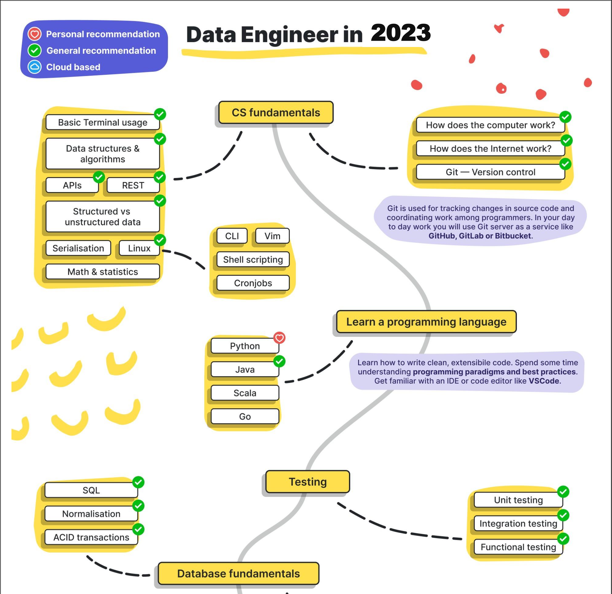
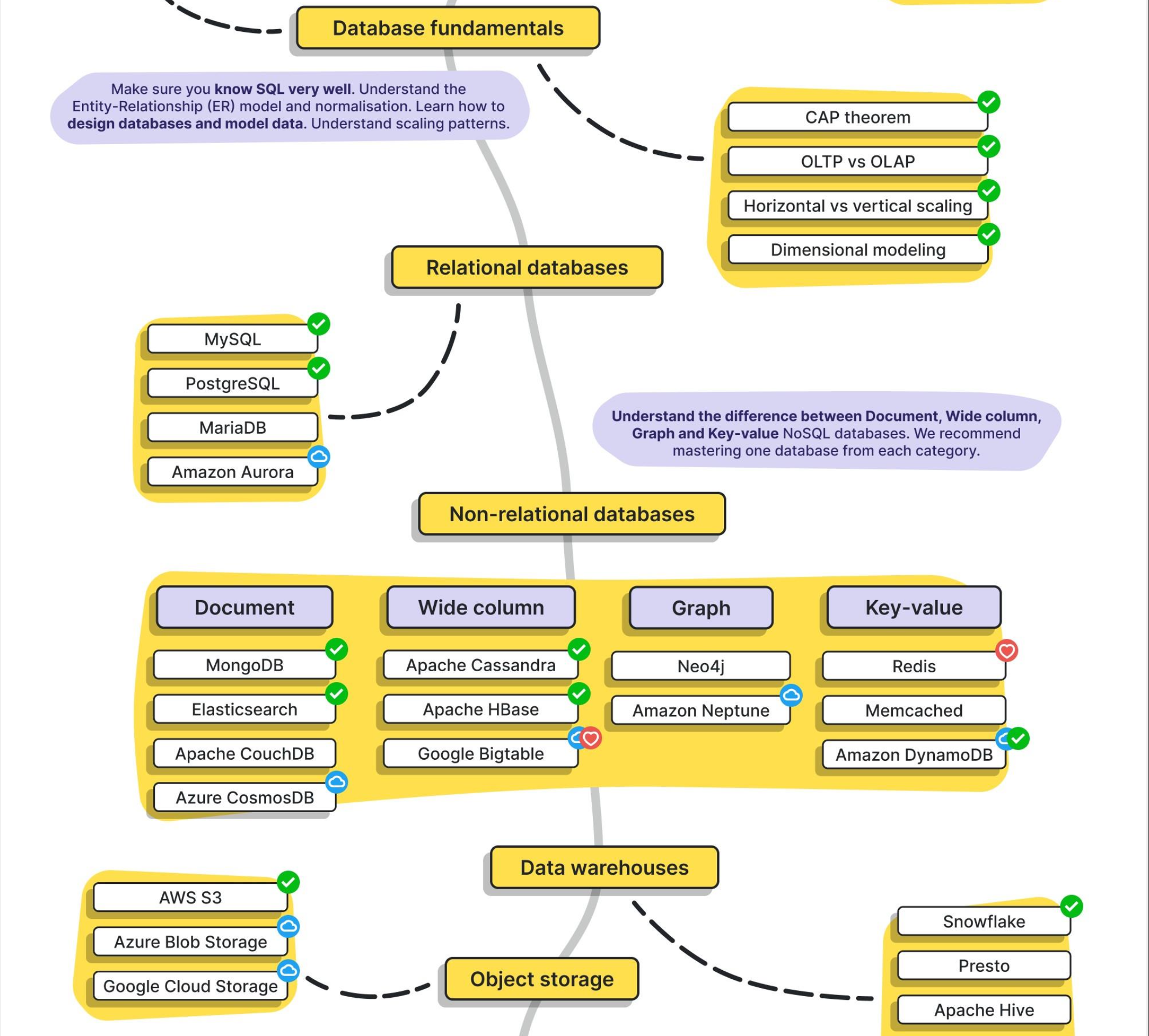
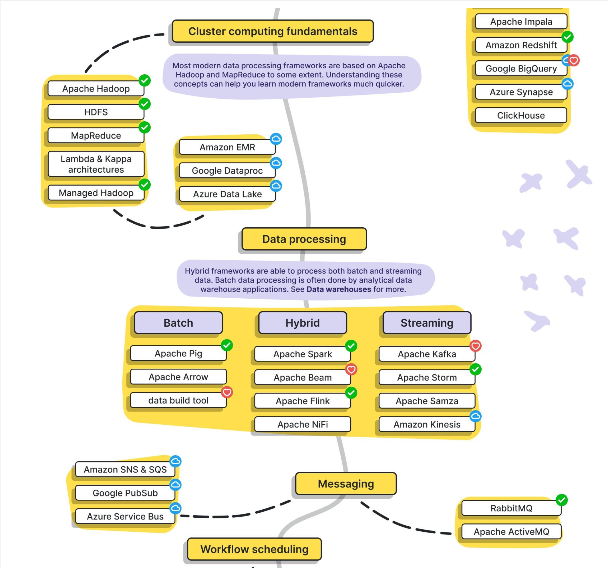
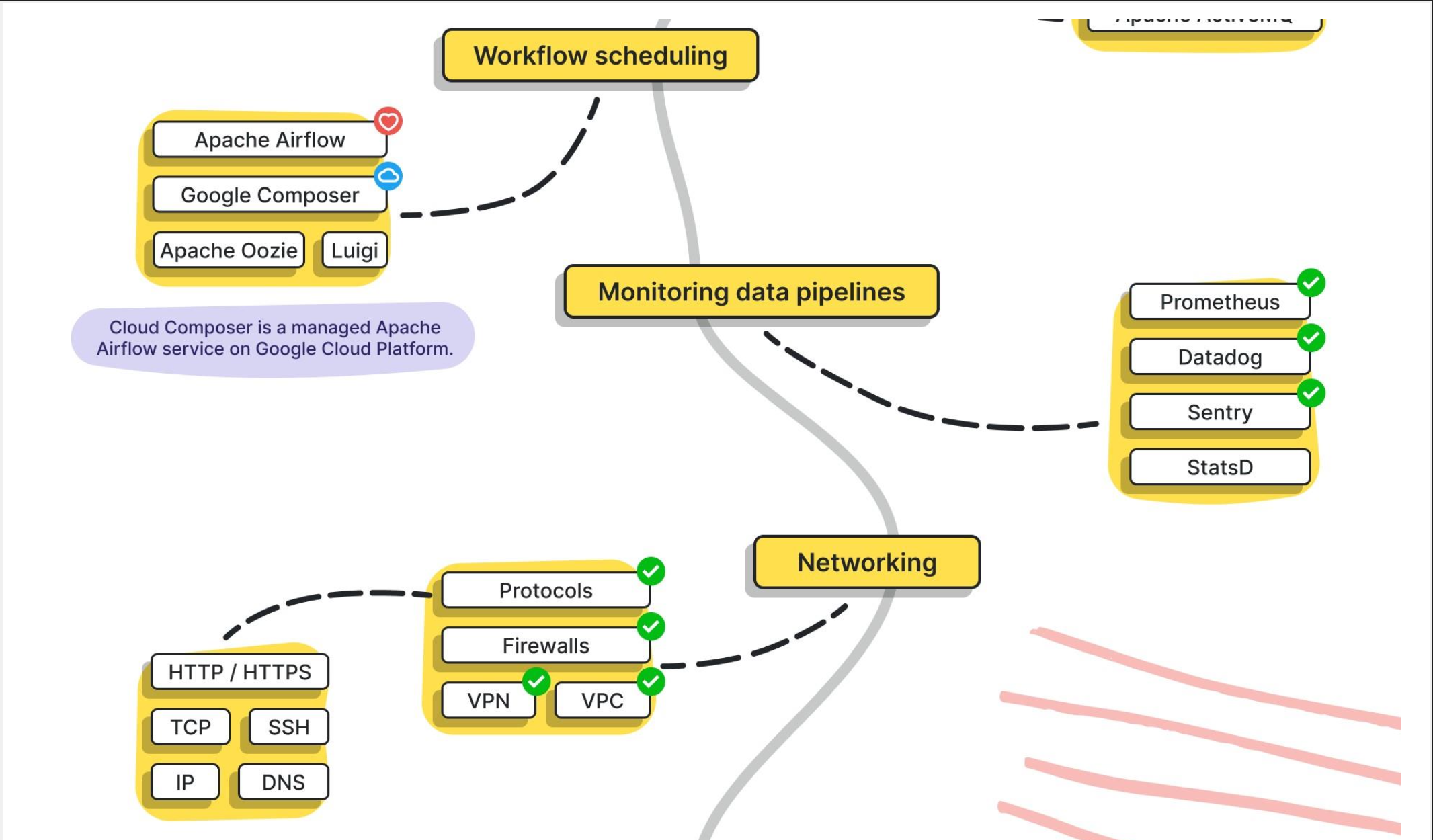
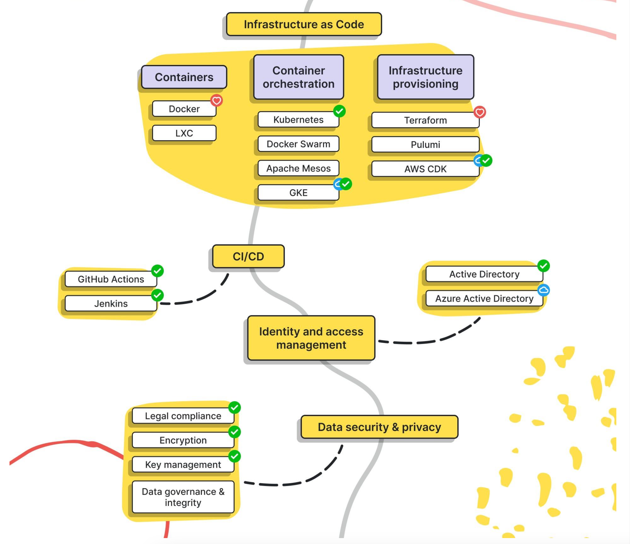
src: https://www.linkedin.com/in/pooja-jain-898253106/
[Avg. reading time: 3 minutes]
Notebooks vs IDE
| Feature | Notebooks (.ipynb) | Python Scripts (.py) |
|---|---|---|
| Use Case - DE | Quick prototyping, visualizing intermediate steps | Production-grade ETL, orchestration scripts |
| Use Case - DS | EDA, model training, visualization | Packaging models, deployment scripts |
| Interactivity | High – ideal for step-by-step execution | Low – executed as a whole |
| Visualization | Built-in (matplotlib, seaborn, plotly support) | Needs explicit code to save/show plots |
| Version Control | Harder to diff and merge | Easy to diff/merge in Git |
| Reusability | Lower, unless modularized | High – can be organized into functions, modules |
| Execution Context | Cell-based execution | Linear, top-to-bottom |
| Production Readiness | Poor (unless using tools like Papermill, nbconvert) | High – standard for CI/CD & Airflow etc. |
| Debugging | Easy with cell-wise changes | Needs breakpoints/logging |
| Integration | Jupyter, Colab, Databricks Notebooks | Any IDE (VSCode, PyCharm), scheduler integration |
| Documentation & Teaching | Markdown + code | Docstrings and comments only |
| Unit Tests | Not practical | Easily written using pytest, unittest |
| Package Management | Ad hoc, via %pip, %conda | Managed via requirements.txt, poetry, pipenv |
| Using Libraries | Easy for experimentation, auto-reloads supported | Cleaner imports, better for dependency resolution |
Tags
abs
/Protocol/Idempotency
ai
/Big Data Overview/Trending Technologies
amazonprime
/Protocol/Monolithic Architecture
amd
/Containers/CPU Architecture Fundamentals
analysis
/Big Data Overview/How does it help?
api
/Protocol/API Performance
apiinbigdata
/Protocol/API in Big Data world
architecture
/Containers/CPU Architecture Fundamentals
arm
/Containers/CPU Architecture Fundamentals
armtemplates
/Cloud Computing/Azure Cloud/IaC
arrow
/Data Format/Arrow
automation
/CLI Tools/JQ
availability
/Big Data Overview/CAP Theorem
avro
/Data Format/Avro
awk
/CLI Tools/AWK
aws
/Cloud Computing/Multi-Cloud
az
/Cloud Computing/Azure Cloud
azure
/Cloud Computing/Azure Cloud
/Cloud Computing/Azure Cloud/Services
/Cloud Computing/Azure Cloud/Terraform
/Cloud Computing/Introduction
/Cloud Computing/Multi-Cloud
azurecli
/Cloud Computing/Azure Cloud/Azure Access
banking
/Protocol/Monolithic Architecture
batch
/Data Engineering/Batch vs Streaming
bigdata
/Big Data Overview/Big Data Challenges
/Big Data Overview/Big Data Concerns
/Big Data Overview/Big Data Tools
/Big Data Overview/Eventual Consistency
/Big Data Overview/How does it help?
/Big Data Overview/Introduction
/Big Data Overview/Job Opportunities
/Big Data Overview/Learning Big Data means?
/Big Data Overview/Optimistic Concurrency
/Big Data Overview/The Big V's
/Big Data Overview/The Big V's/Other V's
/Big Data Overview/The Big V's/Variety
/Big Data Overview/The Big V's/Velocity
/Big Data Overview/The Big V's/Veracity
/Big Data Overview/The Big V's/Volume
/Big Data Overview/Trending Technologies
/Big Data Overview/What is Data?
/Data Format/CSV-TSV
/Data Format/Introduction
/Data Format/JSON
/Data Format/Parquet
bigv
/Big Data Overview/The Big V's
/Big Data Overview/The Big V's/Variety
/Big Data Overview/The Big V's/Velocity
/Big Data Overview/The Big V's/Veracity
/Big Data Overview/The Big V's/Volume
binary
/Big Data Overview/The Big V's/Variety
bronze
/Data Engineering/Medallion Architecture
calc
/CICD/CICD Tools
cap
/Big Data Overview/CAP Theorem
cd
/CICD/CD Yaml
/CICD/Introduction
certification
/Miscellaneous/Additional Reading
challenges
/Cloud Computing/Challenges
chapter1
ci
/CICD/Introduction
cicd
/CICD/CICD Tools
/CICD/Introduction
/Protocol/Microservices
cli
/CLI Tools/JQ
/CLI Tools/Linux Commands 01
/CLI Tools/Linux Commands 02
/Data Format/Duck DB
cloud
/Big Data Overview/Big Data Tools
/Cloud Computing/Challenges
/Cloud Computing/Introduction
cloudnative
/Cloud Computing/Cloud Native vs Lift-and-Shift
columnar
/Big Data Overview/NO Sql Databases
/Data Format/Parquet
commands
/CLI Tools/Linux Commands 01
compressed
/Data Format/Parquet
concerns
/Big Data Overview/Big Data Concerns
concurrent
/Big Data Overview/Concurrent vs Parallel
connectionpool
/Protocol/API Performance
consistency
/Big Data Overview/CAP Theorem
container
/Containers/Docker
/Containers/Docker Examples
/Containers/VMs or Containers
/Containers/What Container does
containers
/Containers/Introduction
continuous
/Big Data Overview/Types of Data
csv
/Data Format/CSV-TSV
csvkit
/CLI Tools/CSV SQL
csvsql
/CLI Tools/CSV SQL
/CLI Tools/CSV SQL
curl
/Protocol/REST API
dask
/Advanced Python/Data Frames
data
/Big Data Overview/What is Data?
dataengineering
/Data Engineering/Introduction
dataformat
/Data Format/Arrow
/Data Format/CSV-TSV
/Data Format/Introduction
/Data Format/JSON
/Data Format/Parquet
/Data Format/YAML
datalake
/Big Data Overview/Data Integration
datamesh
/Data Engineering/Data Mesh
dataquality
/Big Data Overview/Big Data Challenges
/Data Engineering/Data Quality Checks
dbaas
/Cloud Computing/Types of Cloud Services
decorator
/Advanced Python/Decorator
devcontainer
devops
/Cloud Computing/Azure Cloud/Terraform
discrete
/Big Data Overview/Types of Data
distributed
/Big Data Overview/Scaling
docker
/Containers/Docker
/Containers/Docker Examples
/Containers/Introduction
/Containers/VMs or Containers
/Containers/What Container does
dockerhub
/Containers/Docker Examples
documentdb
/Big Data Overview/NO Sql Databases
domain
/Big Data Overview/DSL
domainownership
/Data Engineering/Data Mesh
dr
/Cloud Computing/Disaster Recovery (DR)
dsl
/Big Data Overview/DSL
duckdb
/Data Format/Duck DB
elt
/Big Data Overview/Data Integration
errorhandling
/Advanced Python/Error Handling
ethics
/Big Data Overview/Big Data Challenges
etl
/Big Data Overview/Data Integration
eventhubs
/Data Engineering/KAFKA/Different types of streaming
eventualconsistency
/Big Data Overview/Eventual Consistency
exception
/Advanced Python/Error Handling
faas
/Cloud Computing/Types of Cloud Services
free
/Miscellaneous/Additional Reading
funnel
/Data Engineering/Data Engineering Model
gcp
/Cloud Computing/Multi-Cloud
gdpr
/Data Engineering/Quality & Governance
get
/Protocol/HTTP
gitbash
/CLI Tools/Linux Commands 01
github
/CICD/CI Yaml
githubactions
/CICD/CI Yaml
/CICD/CICD Tools
gold
/Data Engineering/Medallion Architecture
governance
/Data Engineering/Quality & Governance
gpl
/Big Data Overview/GPL
graphdb
/Big Data Overview/NO Sql Databases
grpc
/Protocol/Introduction
ha
/Cloud Computing/High Availability
hierarchical
/Data Format/JSON
highavailability
/Cloud Computing/High Availability
horizontal
/Big Data Overview/Scaling
html
/Big Data Overview/DSL
http
/Protocol/HTTP
/Protocol/Introduction
hub
/Containers/Docker
iaas
/Cloud Computing/Types of Cloud Services
iac
/Cloud Computing/Azure Cloud/IaC
/Cloud Computing/Azure Cloud/Idempotency
idempotency
/Cloud Computing/Azure Cloud/Idempotency
idempotent
/Protocol/Idempotency
image
/Big Data Overview/The Big V's/Variety
info
/Advanced Python/Logging
interoperability
/Big Data Overview/Big Data Challenges
introduction
iot
/Big Data Overview/Trending Technologies
jobs
/Big Data Overview/Job Opportunities
jq
/CLI Tools/JQ
json
/Big Data Overview/The Big V's/Variety
/CLI Tools/JQ
/Data Format/JSON
jwt
/Protocol/Statelessness
kafka
/Big Data Overview/Big Data Tools
/Data Engineering/Batch vs Streaming
/Data Engineering/KAFKA/Introduction
/Data Engineering/KAFKA/Kafka Software
/Data Engineering/KAFKA/Python Scripts
/Data Engineering/KAFKA/Use Cases
/Protocol/API in Big Data world
keyvalue
/Big Data Overview/NO Sql Databases
kinesis
/Data Engineering/KAFKA/Different types of streaming
/Data Engineering/KAFKA/Kafka Software
knowledge
/Big Data Overview/How does it help?
learning
/Big Data Overview/Learning Big Data means?
/Big Data Overview/Learning Big Data means?
library
/CLI Tools/AWK
lift
/Cloud Computing/Cloud Native vs Lift-and-Shift
linkedinlearning
/Miscellaneous/Additional Reading
lint
/Developer Tools/Other Python Tools
linux
/CLI Tools/Linux Commands 01
/CLI Tools/Linux Commands 02
loadbalancer
/Protocol/Statefulness
loadbalancing
/Protocol/API Performance
logging
/Advanced Python/Logging
medallion
/Data Engineering/Medallion Architecture
memoization
/Advanced Python/Decorator
merge
/Protocol/Idempotency
microservices
/Protocol/Microservices
mitigation
/Big Data Overview/Big Data Concerns
monolithic
/Protocol/Monolithic Architecture
mqtt
/Protocol/Introduction
multicloud
/Cloud Computing/Multi-Cloud
mypy
/Developer Tools/Other Python Tools
nominal
/Big Data Overview/Types of Data
nosql
/Big Data Overview/NO Sql Databases
optimistic
/Big Data Overview/Optimistic Concurrency
oracle
/Cloud Computing/Multi-Cloud
ordinal
/Big Data Overview/Types of Data
otherv
/Big Data Overview/The Big V's/Other V's
overview
/Big Data Overview/Introduction
/Cloud Computing/Introduction
paas
/Cloud Computing/Types of Cloud Services
pagination
/Protocol/API Performance
pandas
/Advanced Python/Data Frames
parallelprogramming
/Big Data Overview/Concurrent vs Parallel
parquet
/Data Format/Duck DB
/Data Format/Parquet
parser
/CLI Tools/JQ
partitiontolerant
/Big Data Overview/CAP Theorem
pep
/Developer Tools/Other Python Tools
performance
/Protocol/API Performance
pipeline
/Big Data Overview/Data Integration
/Data Engineering/Introduction
poetry
/Developer Tools/Introduction
polars
/Advanced Python/Data Frames
post
/Protocol/HTTP
privacy
/Big Data Overview/Big Data Challenges
protocols
/Protocol/Introduction
pubsub
/Data Engineering/KAFKA/Kafka Software
put
/Protocol/HTTP
pytest
/Advanced Python/Unit Testing
python
/Big Data Overview/GPL
/Data Engineering/KAFKA/Python Scripts
/Developer Tools/Introduction
qualitative
/Big Data Overview/Types of Data
quantitative
/Big Data Overview/Types of Data
rawdata
/Big Data Overview/Data Integration
/Big Data Overview/How does it help?
rdbms
/Data Format/Introduction
realtime
/Big Data Overview/Big Data Challenges
/Data Engineering/Batch vs Streaming
/Data Engineering/KAFKA/Introduction
region
/Cloud Computing/Azure Cloud
repositories
/Containers/Docker
requests
/Protocol/REST API
rest
/Protocol/REST API
/Protocol/Statelessness
restapi
/Protocol/Microservices
/Protocol/REST API
robotics
/Big Data Overview/Trending Technologies
rowbased
/Data Format/Avro
rpo
/Cloud Computing/Disaster Recovery (DR)
/Cloud Computing/RTO - RPO
rto
/Cloud Computing/Disaster Recovery (DR)
/Cloud Computing/RTO - RPO
ruff
/Developer Tools/Other Python Tools
rust
/Big Data Overview/GPL
/Developer Tools/UV
saas
/Cloud Computing/Types of Cloud Services
scaling
/Big Data Overview/Scaling
schemadrift
/Data Engineering/Data Quality Checks
sdk
/Cloud Computing/Azure Cloud/Azure Access
selfservice
/Data Engineering/Data Mesh
semistructured
/Big Data Overview/The Big V's/Variety
sequence
/Data Engineering/Data Engineering Model
services
/Cloud Computing/Azure Cloud/Services
setup
shift
/Cloud Computing/Cloud Native vs Lift-and-Shift
silver
/Data Engineering/Medallion Architecture
singlefiledatabase
/Data Format/Duck DB
softwares
/Data Engineering/KAFKA/Kafka Software
spark
/Big Data Overview/Big Data Tools
/Protocol/API in Big Data world
sql
/Big Data Overview/DSL
starmodel
/Data Engineering/Data Engineering Model
stateful
/Data Engineering/KAFKA/Different types of streaming
/Protocol/Statefulness
stateless
/Data Engineering/KAFKA/Different types of streaming
statelessness
/Protocol/Statelessness
statuscodes
/Protocol/HTTP
stickiness
/Protocol/Statefulness
storage
/Big Data Overview/Big Data Challenges
streaming
/Data Engineering/Batch vs Streaming
structured
/Big Data Overview/The Big V's/Variety
technologies
/Big Data Overview/Trending Technologies
teraform
/Protocol/Idempotency
terraform
/Cloud Computing/Azure Cloud/IaC
/Cloud Computing/Azure Cloud/Terraform
textbased
/CLI Tools/AWK
tools
/Big Data Overview/Big Data Tools
/CLI Tools/JQ
/Data Format/Duck DB
traditionaldata
/Big Data Overview/What is Data?
try
/Advanced Python/Error Handling
tsv
/Data Format/CSV-TSV
unittesting
/Advanced Python/Unit Testing
unstructured
/Big Data Overview/The Big V's/Variety
upsert
/Protocol/Idempotency
usecases
/Data Engineering/KAFKA/Use Cases
uv
/Developer Tools/Introduction
/Developer Tools/UV
validation
/Data Engineering/Data Quality Checks
validity
/Big Data Overview/The Big V's/Other V's
value
/Big Data Overview/The Big V's/Other V's
velocity
/Big Data Overview/The Big V's/Velocity
venv
/Developer Tools/Introduction
/Developer Tools/UV
veracity
/Big Data Overview/The Big V's/Veracity
version
/Big Data Overview/The Big V's/Other V's
vertical
/Big Data Overview/Scaling
vm
/Containers/VMs or Containers
volume
/Big Data Overview/The Big V's/Volume
webportal
/Cloud Computing/Azure Cloud/Azure Access
worksforme
/Containers/What Container does
workspace
xml
/Big Data Overview/The Big V's/Variety
yaml
/CICD/CD Yaml
/CICD/CI Yaml
/Data Format/YAML
yq
/Data Format/YAML